[CV] Detection

Introduction

Detection是Computer Vision领域一个非常火热的研究方向。并且在工业界也有着十分广泛的应用(例如人脸检测、无人驾驶的行人/车辆检测等等)。本文质旨在梳理RCNN–SPPNet–Fast RCNN–Faster RCNN–FCN–Grid RCNN，YOLO v1/2/3, SSD等Object Detection这些非常经典的工作。

@LucasX注：本文长期更新。

RCNN (Region-based CNN)

Paper: Rich feature hierarchies for accurate object detection and semantic segmentation

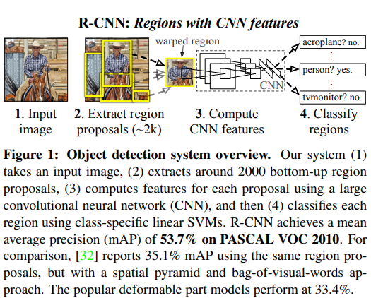
What is RCNN?

这篇Paper可以看做是Deep Learning在Object Detection大获成功的开端，对Machine Learning/Pattern Recognition熟悉的读者应该都知道，Feature Matters in approximately every task! 而RCNN性能提升最大的因素之一便是很好地利用了CNN提取的Feature，而不是像先前的detector那样使用手工设计的feature(例如SIFT/LBP/HOG等)。

RCNN可以认为是Regions with CNN features，即(1)先利用Selective Search算法生成大约2000个Region Proposal，(2)Pretrained CNN从这些Region Proposal中提取deep feature(from pool5)，(3)然后再利用linear SVM进行one-VS-rest分类。从而将Object Detection问题转化为一个Classification问题，对于Selective Search框选不准的bbox，后面使用Bounding Box Regression(下面会详细介绍)进行校准。这便是RCNN的主要idea。

Details of RCNN

Pretraining and Fine-tuning

RCNN先将Base Network在ImageNet上train一个1000 class的classifier，然后将output neuron设置为21(20个Foreground + 1个Background)在target datasets上fine-tune。其中，将由Selective Search生成的Region Proposal与groundtruth Bbox的$IOU\geq 0.5$的定义为positive sample，其他的定义为negative sample。

作者在实验中发现，pool5 features learned from ImageNet足够general，并且在domain-specific datasets上学习non-linear classifier可以获得非常大的性能提升。

Bounding Box Regression

输入是$N$个training pairs，$\{(P^i,G^i)\}_{i=1,2,\cdots,N}, P^i=(P_x^i,P_y^i,P_w^i,P_h^i)$代表$P^i$像素点的$(x,y)$坐标点、width和height。$G=(G_x,G_y,G_w,G_h)$代表groundtruth bbox。BBox Regression的目的就是为了学习一种mapping使得proposed box $P$ 映射到 groundtruth box $G$。

将$x,y$的transformation设为$d_x(P),d_y(P)$，属于scale-invariant translation。$w,h$是log-space translation。学习完成后，可将input proposal转换为predicted groundtruth box $\hat{G}$:
$$
\hat{G}_x=P_w d_x(P)+P_x
$$

$$
\hat{G}_y=P_h d_x(P)+P_y
$$

$$
\hat{G}_w=P_w exp(d_w(P))
$$

$$
\hat{G}_h=P_h exp(d_h(P))
$$

每个$d_{\star}(P)$都用一个线性函数来进行建模，使用$pool_5$ feature，权重的学习则使用OLS优化即可：
$$
w_{\star}=\mathop{argmin} \limits_{\hat{w}_{\star}} \sum_i^N (t_{\star}^i-\hat{w}_{\star}^T \phi_5 (P^i))^2 + \lambda||\hat{w}_{\star}||^2
$$

The regression targets $t_{\star}$ for the training pair $(P, G)$ are defined as:
$$
t_x=\frac{G_x-P_x}{P_w}
$$

$$
t_y=\frac{G_y-P_y}{P_h}
$$

$$
t_w=log(\frac{G_w}{P_w})
$$

$$
t_h=log(\frac{G_h}{P_h})
$$

在选取Proposed Bbox的时候，我们只选取离Groundtruth Bbox比较近的($IOU\geq 0.6$)来做Bounding Box Regression。

以上就是Deep Learning在Object Detection领域一个开创性的工作–RCNN。若有疑问，欢迎给我留言！

SPPNet

Paper: Spatial pyramid pooling in deep convolutional networks for visual recognition.

What is SPPNet?

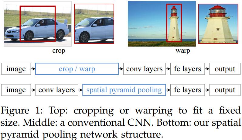
SPPNet(Spatial Pyramid Pooling)是基于RCNN进行改进的一个Object Detection算法。介绍SPPNet之前，我们不妨先来看一下RCNN有什么问题？RCNN，即Region-based CNN，它需要CNN作为base network去做特征提取，而传统CNN需要固定的squared input，而为了满足这个条件，就需要手工地对原图进行裁剪、变形等操作，而这样势必会丢失信息。作者意识到这种现象的原因不在于卷积层，而在于FC Layers需要固定的输入尺寸，因此通过在feature map的SSPlayer可以满足对多尺度的feature map裁剪，从而concatenate得到固定尺寸的特征输入。取得了很好的效果，在detection任务上，region proposal直接在feature map上生成，而不是在原图上生成，因此可以仅仅通过一次特征提取，而不需要像RCNN那样提取2000次(2000个 Region Proposal)，这大大加速了检测效率。

@LucasX注：现如今的Deep Architecture比较多采用Fully Convolutional Architecture(全卷积结构)，而不含Fully Connected Layers，在最后做分类或回归任务时，采用Global Average Pooling即可。

Why SPPNet?

SPPNet创新点在于：

1. SPP可以在不顾input size的情况下获取fixed size output，这是sliding window做不到的。
2. SPP uses multi-level spatial bins，而sliding window仅仅使用single window size。multi-level pooling对object deformation则十分地robust。
3. SPP can pool features extracted at variable scales thanks to the flexibility of input scales.
4. Training with variable-size images increases scale-invariance and reduces over-fitting.

Details of SPPNet

SPP Layer

SPP Layer can maintain spatial information by pooling in local spatial bins. These spatial bins have sizes proportional to the image size, so the number of bins is fixed regardless of the image size. This is in contrast to the sliding window pooling of the previous deep networks,where the number of sliding windows depends on the input size.

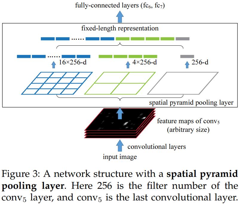
这样，通过不同spatial bin pooling得到的k个 M-dimensional feature concatenation，我们就可以得到fixed length的feature vector了，接下来是不是就可以愉快地用FC Layers/SVM等ML算法train了？

SPP的优点：

1. 能够在给定任意input size的时候依然输出fixed size output
2. multi-level spatial bin，能够capture multi-scale信息（这一点其实非常重要，Inception，以及更近一些的网络结构例如MixNet/SKNet等等都是利用了多尺度信息），multi-level对deformation更robust

既然引入SPP后，网络可以不用受制于fixed size input，那么自然可以用于多尺度训练：第$i$个epoch用input size为$M$进行训练，下一个epoch用input size为$N$进行训练，网络参数对所有variant input size是共享的，以此来使得模型对multi-scale object更加robust。

SPP for Detection

RCNN需要从2K个Region Proposal中feedforwad Pretrained CNN去提取特征，这显然是非常低效的。SPPNet直接将整张image(possible multi-scale)作为输入，这样就可以只feedforwad一次CNN。然后在feature map层面获取candidate window，SPP Layer pool到fixed-length feature representation of the window。

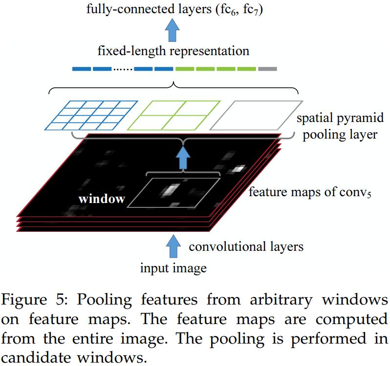
Region Proposal生成阶段和RCNN比较相似，将原始image resize使得$min(w, h)=s$，Selective Search/EdgeBox等算法生成2000个bbox candidate，文中采用 4-level spatial pyramid ($1\times 1, 2\times 2, 3\times 3,6\times 6$, totally 50 bins) to pool the features。对于每个window，该Pooling操作得到一个12800-Dimensional (256×50) 的向量。这个向量作为FC Layers的输入，然后和RCNN一样训练linear SVM去做分类。

训练SPP Detector时，正负样本的采样是基于groundtruth bbox为基准，$IOU\geq 0.3$为positive sample，反之为negative sample。

Mapping a Window to Feature Maps

补充一下SPPNet是如何在feature map上做映射的，因为这个算法比较古老了，而且也比较好懂，就不赘述了，贴一下原文吧：

In the detection algorithm (and multi-view testing on feature maps), a window is given in the image domain, and we use it to crop the convolutional feature maps (e.g., conv5) which have been sub-sampled several times. So we need to align the window on the feature maps. In our implementation, we project the corner point of a window onto a pixel in the feature maps, such that this corner point in the image domain is closest to the center of the receptive field of that feature map pixel. The mapping is complicated by the padding of all convolutional and pooling layers. To simplify the implementation, during deployment we pad $\lfloor p/2 \rfloor$, pixels for a layer with a filter size of p. As such, for a response centered at $(x^{‘}, y^{‘})$, its effective receptive field in the image domain is centered at $(x, y)=(Sx^{‘}, Sy^{‘})$. where $S$ is the product of all previous strides. In our models, $S = 16$ for ZF-5 on conv5, and $S = 12$ for Overfeat-5/7 on conv5/7. Given a window in the image domain, we project the left (top) boundary by: $x^{‘}=\lfloor x/S \rfloor + 1$ and the right (bottom) boundary $x^{‘}=\lceil x/S \rceil - 1$. If the padding is not $\lfloor p/2 \rfloor$, we need to add a proper offset to $x$.

Fast RCNN

Paper: Fast RCNN

Fast RCNN是Object Detection领域一个非常经典的算法。它的novelty在于引入了两个branch来做multi-task learning(category classification和bbox regression)。

Why Fast RCNN?

按照惯例，我们不妨先来看一看之前的算法(RCNN/SPPNet)有什么缺点？

1. 它们(RCNN/SPP)的训练都属于multi-stage pipeline，即先要利用Selective Search生成2K个Region Proposal，然后用log loss去fine-tune一个deep CNN，用Deep CNN抽取的feature去拟合linear SVM，最后再去做Bounding Box Regression。
2. 训练很费时，CNN需要从每一个Region Proposal抽取deep feature来拟合linear SVM。
3. testing的时候慢啊，还是太慢了。因为需要将Deep CNN抽取的feature先缓存到磁盘，再读取feature来拟合linear SVM，你说麻烦不麻烦。

那我们再来看看Fast RCNN为什么优秀？

1. 设计了一个multi-task loss，来同时优化object classification和bounding box regression。
2. Training is single stage.
3. Higher performance than RCNN and SPPNet.

Details of Fast RCNN

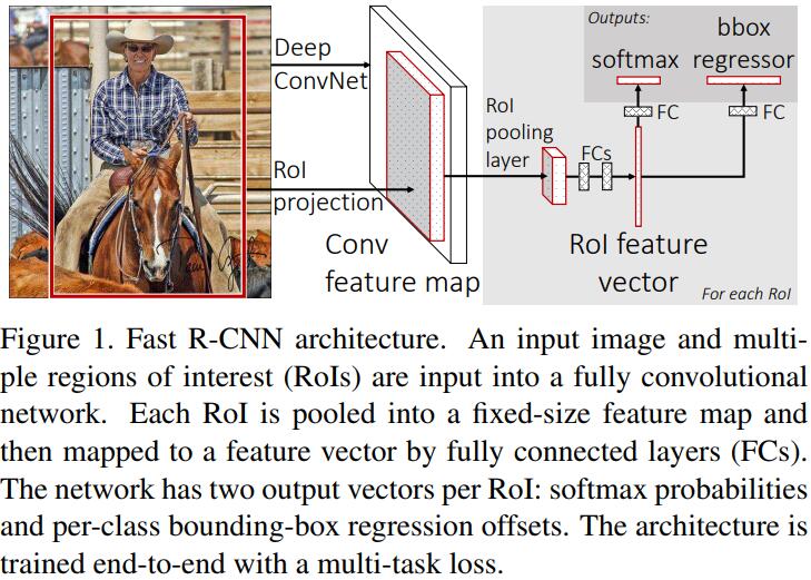
Fast RCNN pipeline如上图所示：它将whole image with several object proposals作为输入，CNN抽取feature，对于每一个object proposal，region of interest (RoI) pooling layer extracts a fixed-length feature vector from the feature map，然后将走过RoI Pooling Layer的feature vector输送到随后的multi-branch，一同做classification和bbox regression。

可以看到，Fast RCNN模型里面一个非常重要的组件叫做RoI Pooling，那么接下来我们就来细细分析一下RoI Pooling究竟是何方神圣。

The RoI pooling layer

Fast RCNN原文里是这样说的：

RoI pooling layer uses max pooling to convert the features inside any valid region of interest into a small feature map with a fixed spatial extent of $H\times W$ (e.g., $7\times 7$), where $H$ and $W$ are layer hyper-parameters that are independent of any particular RoI.

In this paper, an RoI is a rectangular window into a conv feature map. Each RoI is defined by a four-tuple $(r, c, h, w)$ that specifies its top-left corner $(r, c)$ and its height and width $(h, w)$.

RoI max pooling works by dividing the $h\times w$ RoI window into an $H\times W$ grid of sub-windows of approximate size $h/H \times w/W$ and then max-pooling the values in each sub-window into the corresponding output grid cell. Pooling is applied independently to each feature map channel, as in standard max pooling. The RoI layer is simply the special-case of the spatial pyramid pooling layer used in SPPnets [11] in which there is only one pyramid level. We use the pooling sub-window calculation given in [11].

什么意思呢？就是在任何valid region proposal里面，把某层的feature map划分成多个小方块，每个小方块做max pooling，这样就得到了尺寸更小的feature map。

Fine-tuning for detection

Multi-Task Loss

之前也说过，Fast RCNN同时做了$K+1$ (K个object class + 1个background) 类的classification($p=(p_0,p_1,\cdots,p_K)$)和bbox regression($t^k = (t^k_x, t^k_y, t^k_w, t^k_h)$)。

We use the parameterization for $t^k$ given in [9], in which $t^k$ specifies a scale-invariant translation and log-space height/width shift relative to an object proposal(对linear regression熟悉的读者不妨思考一下为什么要对width和height做log). Each training RoI is labeled with a ground-truth class $u$ and a ground-truth bounding-box regression target $v$. We use a multi-task loss $L$ on each labeled RoI to jointly train for classification and bounding-box regression:
$$
L(p,u,t^u,v)=L_{cls}(p,u)+\lambda [u\geq1]L_{loc}(t^u,v)
$$
$L_{cls}(p,u)=-logp_u$ is log loss for true class $u$.

我们再来看看Loss Function的第二部分(即regression loss)，$[u\geq 1]$代表只有满足$u\geq 1$时这个式子才为1，否则为0。在我们的setting中，background的$[u\geq 1]$自然而然就设为0啦。我们接着分析regression loss，既然是regression，惯常的手法是使用MSE Loss对不对？但是MSE Loss属于Cost-sensitive Loss啊，对outliers非常的敏感，因此Ross使用了更加柔和的$Smooth L_1 Loss$。
$$
L_{loc}(t^u,v)\sum_{i\in \{x,y,w,h\}} smooth_{L_1}(t_i^u-v_i)
$$

Smooth L1 Loss写得详细一点呢，就是这样的：
$$
smooth_{L_1}(x)=
\begin{cases}
0.5x^2 & if |x|<1\\
|x|-0.5 & otherwise
\end{cases}
$$

@LucasX注：想详细了解Machine Learning中的Loss，请参考我的另一篇文章。

Mini-batch sampling

在Fine-tuning阶段，每个mini-batch随机采样自$N=2$类image，每一类都是64个sample，与groundtruth bbox $IOU\geq 0.5$的设为foreground samples[$u=1$]，反之为background samples[$u=0$]。

Fast R-CNN detection

因为Fully Connected Layers的计算太费时，而FC Layers的计算显然就是大矩阵相乘，因此很容易联想到用truncated SVD来进行加速。

In this technique, a layer parameterized by the $u\times v$ weight matrix $W$ is approximately factorized as:
$$
W\approx U\Sigma_t V^T
$$
$U$是由$W$前$t$个left-singular vectors组成的$u\times t$矩阵，$\Sigma_t$是包含$W$矩阵前$t$个singular value的$t\times t$对角矩阵，$V$是由$W$前$t$个right-singular vectors组成的$v\times t$矩阵。Truncated SVD可以将参数从$uv$降到$t(u+v)$。

这里值得一提的有两点：

1. $conv_1$ layers feature map通常都足够地general，并且task-independent。因此可以直接用来抽feature就行。
2. Region Proposal的数量对Detection的性能并没有什么太大影响 (关键还是看feature啊！以及sampling mini-batch的时候正负样本的不均衡问题，详情请参阅kaiming He大神的Focal Loss)。

Faster RCNN

Paper: Faster r-cnn: Towards real-time object detection with region proposal networks

Faster RCNN也是Object Detection领域里一个非常具有代表性的工作，一个最大的改进就是Region Proposal Network(RPN)，RPN究竟神奇在什么地方呢？我们先来回顾一下RCNN–SPP–Fast RCNN，这些都属于two-stage detector，什么意思呢？就是先利用Selective Search生成2000个Region Proposal，然后再将其转化为一个机器学习中的分类问题。而Selective Search实际上是非常低效的，RPN则很好地完善了这一点，即直接从整个Network Architecture里生成Region Proposal。RPN是一种全卷积网络，它可以同时预测object bounds，以及objectness score。因为RPN的Feature是和Detection Network共享的，所以整个Region Proposal的生成几乎是cost-free的。所以，这也就是Faster RCNN中Faster一词的由来。

What is Faster RCNN?

$$
Faster RCNN = Fast RCNN + RPN
$$
按照惯例，一个算法的提出显然是为了解决之前算法的不足。那之前的算法都有什么问题呢？
如果对之前的detector熟悉的话，shared features between proposals已经被解决，但是Region Proposal的生成变成了最大的计算瓶颈。这便是RPN产生的缘由。

作者注意到，conv feature maps used by region-based detectors也可以被用于生成region proposals。在这些conv features顶端，通过添加两个额外的卷积层来构造RPN：一个conv layer用于encode每个conv feature map position到一个低维向量(256-d)；另一个conv layer在每一个conv feature map position中输出k个region proposal with various scales and aspect ratios的objectness score和regression bounds。下面重点介绍一下RPN。

Region Proposal Network

RPN是一个全卷积网络，可以接受任意尺寸的image作为输入，并且输出一系列object proposals以及其对应的objectness score。那么RPN是如何生成region proposals的呢？

首先，在最后一个shared conv feature map上slide一个小网络，这个小网络全连接到input conv feature map上$n\times n$的spatial window。而每一个sliding window映射到一个256-d的feature vector，这个feature vector输入到两个fully connected layers–一个做box regression，另一个做box classification。值得注意的是，因为这个小网络是以sliding window的方式操作的，所以fully-connected layers在所有的spatial locations都是共享的。该结构由一个$n\times n$ conv layer followed by two sibling $1\times 1$ conv layers组成。

Translation-Invariant Anchors

对于每个sliding window location，同时预测$k$个region proposals，所以regression layer有$4k$个encoding了$k$个bbox坐标的outputs。classification layer有$2k$个scores(每个region proposal估计object/non-object的概率)。

The $k$ proposals are parameterized relative to $k$ reference boxes, called anchors. Each anchor is centered at the sliding window in question, and is associated with a scale and aspect ratio.

文章中采用3个scales和3个aspect ratios，所以每个sliding position一共得到$k=9$个anchors。所以对于每个$W\times H$的conv feature map一共产生$WHk$个anchor。这种方法一个很重要的性质就是它是translation invariant。

A Loss Function for Learning Region Proposals

训练RPN时，我们为每一个anchor分配binary class(即是不是一个object)。我们为以下这两类anchors分配positive label:

1. 与groundtruth bbox有最高IoU的anchor
2. 与任意groundtruth bbox $IoU\geq 0.7$的anchor

同时，可能出现一个groundtruth bbox分配到多个anchor的情况，我们将与所有groundtruth bbox $IoU\leq 0.3$的anchor设为negative anchor。而那些既不是positive又不是negative的anchor则对training过程没有用处。然后，Faster RCNN的Loss Function就变成：
$$
L(\{p_i\},\{t_i\})=\frac{1}{N_{cls}} \sum_i L_{cls}(p_i,p_i^{\star}) + \lambda \frac{1}{N_{reg}} \sum_i p_i^{\star} L_{reg}(t_i,t_i^{\star})
$$
$p_i$是anchor $i$ 被预测为是一个object的概率，若anchor为positive，则groundtruth label $p_i^{\star}$为1；若anchor为negative则为0；$t_i$是包含4个预测bbox坐标点的向量，$t_i^{\star}$是groundtruth positive anchor坐标点的向量。$L_{cls}$是二分类的Log Loss(object VS non-object)。对于regression loss，文章使用$L_{reg}(t_i,t_i^{\star})=R(t_i-t_i^{\star})$，其中$R$是Smooth L1 Loss(和Fast RCNN中一样)。$p_i^{\star} L_{reg}$表示仅仅在positive anchor ($p_i^{\star}=1$)时才被激活，否则($p_i^{\star}=0$)不激活。

Bounding Box Regression依旧是采用之前的pipeline：
$$
t_x=\frac{x-x_a}{w_a},t_y=\frac{y-y_a}{h_a},t_w=log(\frac{w}{w_a}),t_h=log(\frac{h}{h_a})
$$

$$
t_x^{\star}=\frac{x^{\star}-x_a}{w_a},t_y^{\star}=\frac{y^{\star}-y_a}{h_a},t_w^{\star}=log(\frac{w^{\star}}{w_a}),t_h^{\star}=log(\frac{h^{\star}}{h_a})
$$

In our formulation, the features used for regression are of the same spatial size $(n\times n)$ on the feature maps. To account for varying sizes, a set of $k$ bounding-box regressors are learned. Each regressor is responsible for one scale and one aspect ratio, and the $k$ regressors do not share weights. As such, it is still possible to predict boxes of various sizes even though the features are of a fixed size/scale.

Sharing Convolutional Features for Region Proposal and Object Detection

1. Fine-tune在ImageNet上Pretrain的RPN来完成region proposal task。
2. 利用RPN生成的region proposal来train Fast RCNN。注意在这一步骤中RPN和Faster RCNN没有共享卷积层。
3. 利用detector network来初始化RPN训练，但是我们fix shared conv layers，仅仅fine-tune单独属于RPN的层。注意在这一步骤中RPN和Fast RCNN共享了卷积层。
4. Fix所有shared conv layers，fine-tune Fast RCNN的fc layers。至此，RPN和Fast RCNN共享卷积层，并且形成了一个unified network。

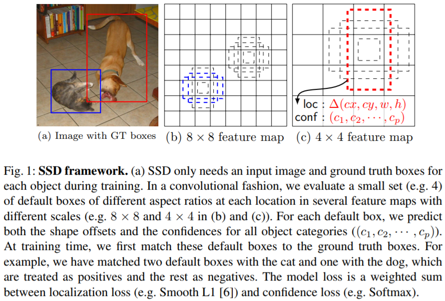
SSD

Paper: SSD: Single Shot MultiBox Detector

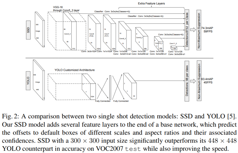
SSD是one-stage detector里一个非常著名的算法，那什么叫做one-stage和two-stage呢？回想一下，从DL Detector发展到现在，我们之前介绍的RCNN/SSP/Fast RCNN/Faster RCNN等，都是属于two-stage detectors，意思就是说第一步需要生成region proposals，第二步再将整个detection转化为对这些region proposals的classification问题来做。那所谓的one-stage detection就自然是不需要生成region proposals了，而是直接输出bbox了。Faster RCNN里面作者已经分析了，two-stage detection为啥慢？很大原因就是因为region proposal generation太慢了(例如Selective Search算法)，所以提出了RPN来辅助生成region proposals。

What is SSD?

SSD最主要的改进就是使用了一个小的Convolution Filter来预测object category和bbox offset。那如何处理多尺度问题呢？SSD采取的策略是将这些conv filter应用到多个feature map上，来使得整个模型对Scale Invariant。

Details of SSD

SSD主要部件如下：一个DCNN用来提取feature，产生fixed-size的bbox以及这些bbox中每个类的presence score，然后NMS用来输出最后的检测结果。Feature Extraction部分和普通的分类DCNN没啥太大的区别，作者在后面新添加了新的结构：

1. Multi-scale feature maps for detection: 在base feature extraction network之后额外添加新的conv layers(所以得到了multi-scale的feature maps)，来使得模型可以处理multi-scale的detection。
2. Convolutional predictors for detection: 每一个新添加的feature layer可以基于small conv filters产生fixed-size detection predictions。
3. Default boxes and aspect ratios: 对于每个feature map cell，算法给出cell中default box的relative offset，以及class-score(表示在每个box中一个class instance出现的概率)。具体的，对于每个given location的$k$个box，产生4个bbox offset和$c$个class score，这样就对每个feature map location上产生了$(c+4)k$个filters，那么对于一个$m\times n$的feature map，则产生$(c+4)kmn$个output。这个做法和Faster RCNN中的anchor box有点类似，但是SSD中将它用到了多个不同resolution的feature map上，因此多个feature map的不同default box shape使得我们可以很高效地给出output box shape。

Training of SSD

前面已经提到了，SSD会在default box周围生成一系列varied location/ratio/scale的boxes，那么到底哪一个box才是和groundtruth真正匹配的呢？作者采用了这样的一个Matching Strategy: 对于每一个groundtruth box，我们从default boxes中选择不同location/ratio/scale的boxes，然后计算它们和任意一个groundtruth box的Jaccard Overlap，并挑选出超过阈值的boxes。那么SSD最终的Loss就可以写成：
$$
L(x,c,l,g)=\frac{1}{N}(L_{conf}(x,c) + \alpha L_{loc}(x,l,g))
$$
其中$N$代表matched default boxes的数量，Localisation Loss和Faster RCNN一样也选择了Smooth L1。$x_{ij}^p=\{0,1\}$为第$i$个default box是否和第$j$个groundtruth box匹配的indicator。
$$
L_{loc}(x,l,g)=\sum_{i\in Pos} \sum_{m\in \{cx,cy,w,h\}}x_{ij}^k smoothL_1(l_i^m-\hat{g}_j^m)
$$

$$
\hat{g}_j^{cx}=(g_j^{cx}-d_i^{cx})/d_i^w
$$

$$
\hat{g}_j^{cy}=(g_j^{cy}-d_i^{cy})/d_i^h
$$

$$
\hat{g}_j^w=log(\frac{g_j^w}{d_i^w})
$$

$$
\hat{g}_j^h=log(\frac{g_j^h}{d_i^h})
$$

Confidence Loss采用Softmax Loss:
$$
L_{conf}(x, c)=-\sum_{i\in Pos}^N x_{ij}^p log(\hat{c}_i^0)-\sum_{\in Neg}log(\hat{c}_i^0)
$$
其中，$\hat{c}_i^p=\frac{exp(c_i^p)}{\sum_p exp(c_i^p)}$

SSD在检测large object时效果很好，但是在检测small object时则效果比较差，这是因为在higher layers，feature map包含的small object信息太少，可通过将input size由$300\times 300$改为$512\times 512$，Zoom Data Augmentation(即采用zoom in来生成large objects, zoom out来生成small objects)来进行一定程度的缓解。

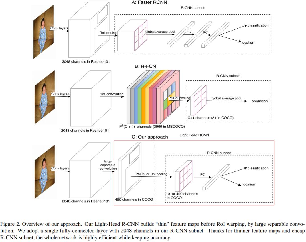
Light-head RCNN

Paper: Light-Head R-CNN: In Defense of Two-Stage Object Detector

Introduction

在介绍Light-head RCNN之前，我们先来回顾一下常见的two-stage detector为什么是heavy-head？作者发现two-stage detector之所以慢，就是因为two-stage detector在RoI Warp前/后 会进行非常密集的计算，例如Faster RCNN包含2个fully connected layers做nRoI Recognition，RFCN会生成很大的score maps。所以无论你的backbone network使用了多么精巧的小网络结构，但是总体速度还是提升不上去。所以针对这个问题，作者在本文提出了light-head RCNN。所谓的light-head，其实说白了就是使用thin feature map + cheap RCNN subnet (pooling和单层fully connected layer)。

大家都知道，two-stage detector，其实是将detection问题转化为一个classification问题来完成的。也就是说，在第一个stage，模型会生成很多region proposal (此为body)，然后在第二个stage对这些region proposal进行分类 (此为head)。通常，two-stage detector的accuracy要比one-stage detector高的，所以为了accuracy，head往往会设计得非常heavy。Light-head RCNN是这么做的：

In this paper, we propose a light-head design to build an efficient yet accurate two-stage detector. Specifically, we apply a large-kernel separable convolution to produce “thin” feature maps with small channel number ($\alpha \times p\times p$ is used in our experiments and $\alpha\leq 10$). This design greatly reduces the computation of following RoI-wise subnetwork and makes the detection system memory-friendly. A cheap single fully-connected layer is attached to the pooling layer, which well exploits the feature representation for classification and regression.

Delve Into Light-Head RCNN

RCNN Subnet

Faster R-CNN adopts a powerful R-CNN which utilizes two large fully connected layers or whole Resnet stage 5 [28, 29] as a second stage classifier, which is beneficial to the detection performance. Therefore Faster R-CNN and its extensions perform leading accuracy in the most challenging benchmarks like COCO. However, the computation could be intensive especially when the number of object proposals is large. To speed up RoI-wise subnet, R-FCN first produces a set of score maps for each region, whose channel number will be $classes_num\times p \times p$ ($p$ is the followed pooling size), and then pool along each RoI and average vote the final prediction. Using a computation-free R-CNN subnet, R-FCN gets comparable results by involving more computation on RoI shared score maps generation.

Faster RCNN虽然在RoI Classification上表现得很好，但是它需要global average pooling来减小第一个fully connected layer的计算量，而GAP会影响spatial localization。此外，Faster RCNN对每一个RoI都要feedforward一遍RCNN subnet，所以在当proposal的数量很大时，效率就非常低了。

Thin Feature Maps for RoI Warping

在feed region proposal到RCNN subnet之前，用RoI warping来得到fixed shape的feature maps。本文提出的light-head产生了一系列thin feature maps，然后再接RoI Pooling层。在实验中，作者发现RoI warping on thin feature maps不仅仅提高了精度，而且节省了training和inference的时间。而且，如果直接应用RoI pooling到thin feature maps上，一方面模型可以减少计算量，另一方面可以去掉GAP来保留spatial information。

Experiments

作者在实验中发现，regression loss比classification loss要小很多，所以将regression loss的权重进行double来balance multi-task training。

YOLO v1

Paper: You Only Look Once: Unified, Real-Time Object Detection

YOLO是One-stage Detection领域里一个非常著名的算法，本文对其V1版本做一个简介。
和基于Slide Window/Region Proposal based two-stage detection不同的是，YOLO可以将整张图作为输入（相比之下，two-stage detector需要在第一步先基于selective search等算法生成region proposal，再基于这些region proposal去做classification），因此YOLO可以获取context information，而Fast RCNN则很容易将background patch误识为object，原因就在于基于region proposal的detector不能获知larger context information。而YOLO则可以很好地解决该问题。

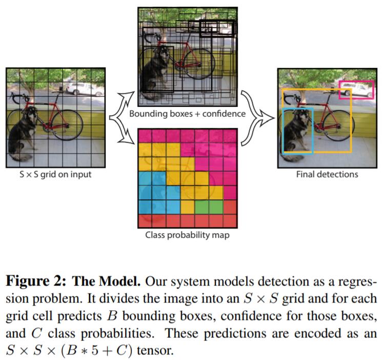
What is YOLO?

YOLO将input image先划分为$S\times S$个grid，若某个object的中心落在了一个grid cell，那么该grid cell就“负责”检测该物体。每个grid cell预测$B$个bbox以及相对应的confidence score，我们将confidence定义为：
$$
Pr(Object)\star IOU_{pred}^{truth}
$$
若该grid cell没有object，则confidence score自然就为0了，confidence score为prediction bbox与gt bbox的IOU。

此外，每个grid cell也预测$C$个conditional class probabilities $Pr(Class_i|Object)$，在测试阶段，我们将conditional class probability和bbox confidence score相乘：
$$
Pr(Class_i|Object)\times Pr(Object)\times IOU_{pred}^{truth}=Pr(Class_i)\times IOU_{pred}^{truth}
$$
这样就得到了对每个box的class-specific confidence score，即同时encode了object在该box中的probability和bbox prediction的精度。

Training of YOLO

因detection需要非常细粒度的feature，所以作者将input resolution由$224\times 224$提升至$448\times 448$来使得网络可以更好地捕捉到细节特征。同时将bbox width/height除以image width/height来进行归一化到$[0, 1]$区间。

We optimize for sum-squared error in the output of our model. We use sum-squared error because it is easy to optimize however it does not perfectly align with our goal of maximizing average precision. It weights localization error equally with classification error which may not be ideal. Also, in every image many grid cells do not contain any object. This pushes the confidence scores of those cells towards zero, often overpowering the gradient from cells that do contain objects. This can lead to model instability, causing training to diverge early on.

针对上述问题，作者使用了两个hyper-param $\lambda_{coord}=5$和$\lambda_{noobj}=0.5$来控制bbox no-object prediction loss和confidence loss。

Sum-squared error also equally weights errors in large boxes and small boxes. Our error metric should reflect that small deviations in large boxes matter less than in small boxes. To partially address this we predict the square root of the bounding box width and height instead of the width and height directly.

YOLO的Loss如下：
$$
\lambda_{coord}\sum_{i=0}^{S^2} \sum_{j=0}^{B}\mathbb{I} _{ij}^{obj}[(x_i-\hat{x}_i)^2+(y_i-\hat{y}_i)^2]
$$

$$
+\lambda_{coord}\sum_{i=0}^{S^2} \sum_{j=0}^{B}\mathbb{I} _{ij}^{obj}[(\sqrt{w_i}-\sqrt{\hat{w}_i})^2+ (\sqrt{h_i}-\sqrt{\hat{h}_i})^2]
$$

$$
+\sum_{i=0}^{S^2} \sum_{j=0}^{B}\mathbb{I}_{ij}^{obj}(C_i-\hat{C}_i)^2 + \lambda_{noobj}\sum_{i=0}^{S^2} \sum_{j=0}^{B}\mathbb{I}_{ij}^{noobj}(C_i-\hat{C}_i)^2
$$

$$
+\sum_{i=0}^{S^2}\mathbb{I}_{i}^{obj}\sum_{c\in classes} (p_i(c)-\hat{p}_i(c))^2
$$

where $\mathbb{I}_{i}^{obj}$ denotes if object appears in cell $i$ and denotes that the $j$-th bounding box predictor in cell $i$ is responsible for that prediction.

Note that the loss function only penalizes classification error if an object is present in that grid cell (hence the conditional class probability discussed earlier). It also only penalizes bounding box coordinate error if that predictor is responsible for the ground truth box (i.e. has the highest IOU of any predictor in that grid cell). However, some large objects or objects near the border of multiple cells can be well localized by multiple cells. Non-maximal suppression can be used to fix these multiple detections.

Limitations of YOLO

Our model also uses relatively coarse features for predicting bounding boxes since our architecture has multiple downsampling layers from the input image. Finally, while we train on a loss function that approximates detection performance, our loss function treats errors the same in small bounding boxes versus large bounding boxes. A small error in a large box is generally benign but a small error in a small box has a much greater effect on IOU. Our main source of error is incorrect localizations.

YOLO V2

YOLO9000: Better, Faster, Stronger.

前面我们已经介绍过YOLO V1，本篇来介绍一下它的改进版本——YOLO V2。YOLO V2也叫YOLO 9000，意思就是说它可以检测9000种object。我们知道，detection的benchmark和classification的benchmark相比，标注成本要更为昂贵(因为画框框远比打标签要麻烦)，而YOLO 9000使用了一种joint training的方法，可以从其他数据集中学习object classification label。此外，和SSD一样，YOLO 9000也使用了multi-scale training来使得它对scale variance更加鲁棒。

Better

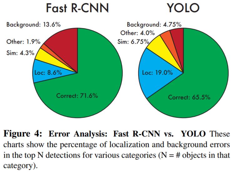
如果大家对YOLO V1还有印象，就会知道作者在对比了YOLO V1和Fast RCNN的error analysis之后，发现YOLO V1的localisation error比较高，并且和基于region-proposal的two-stage detector(例如RCNN系列)相比，recall比较低。所以YOLO V2就主要来解决这两个问题了。

YOLO V2用到了一下几个tricks：

• Batch Normalization: 这个就不多解释了，基本已经成为deep learning models的必备组件。
• High Resolution Classifier: YOLO V2首先在ImageNet上用$448\times 448$ input pretrain 10 epochs，来使得网络的filter对high resolution input更好。
• Convolutional With Anchor Boxes: 这一点idea来源于Faster RCNN，YOLO直接通过FC layer回归bbox coordinates。而Faster RCNN中，RPN可以直接预测anchor boxes的offsets和confidences，因RPN是一个小型的conv net，所以可以在feature map的每一个location预测offsets，而非coordinates。而预测offsets要比coordinates更加方便，同时模型也更容易学习。因此，YOLO V2直接去除了FC layers，并且使用anchor boxes来预测bbox。首先去除了一个Pooling层，来得到高分辨率的输出。其次，输入也由$448\times 448$ 改为$416\times 416$，使用416分辨率的输入是为了保证从得到奇数个的locations，从而保证只有一个center cell。对于large objects而言，很容易占据满image的中间，所以更好的方式是用一个single center location来预测objects，而非其相邻的4个位置。YOLO的卷积层会对input image进行32倍的downsampling，所以使用$416\times 416$的input，我们最终会得到$13\times 13$的feature map。和YOLO V1一样，objectness prediction依然是预测groundtruth和proposed box的IOU，class prediction预测当该bbox为object时，该object所属类别的条件概率。
• Dimension Cluster: YOLO V2在training set bbox上使用KMeans来自动寻找good prior。

• Direct location prediction: 在YOLO中使用anchor box时，我们会碰到model instability问题，尤其是在前几轮的迭代中。这些instability大多来自预测box的位置$(x,y)$。在RPN中，预测值$t_x$、$t_y$、$(x,y)$center coordinate计算方式如下：
  $$
  x=(t_x\times w_a)-x_a
  $$

  $$
  y=(t_y\times h_a)-y_a
  $$

  For example, a prediction of $t_x = 1$ would shift the box to the right by the width of the anchor box, a prediction of $t_x = −1$ would shift it to the left by the same amount.

  YOLO V2采取了V1的做法，预测相对于grid cell的location coordinate值，这样可以将groundtruth限制在0~1之间，作者使用Logistic activation来达到这种效果。

  在output feature map的每个cell中，网络预测出了5个bounding boxes，对于每个bounding box有5个coordinates: $t_x, t_y, t_w, t_h, t_o$。

  If the cell is offset from the top left corner of the image by $(c_x, c_y)$ and the bounding box prior has width and height $p_w, p_h$, then the predictions correspond to:

  $$
  b_x=\sigma(t_x)+c_x
  $$

  $$
  b_y=\sigma(t_y)+c_y
  $$

  $$
  b_w=p_we^{t_w}
  $$

  $$
  b_h=p_he^{t_h}
  $$

  $$
  Pr(object)\times IOU(b, object)=\sigma(t_o)
  $$
  因限制了location prediction，所以参数更容易学习了，模型也更稳定了。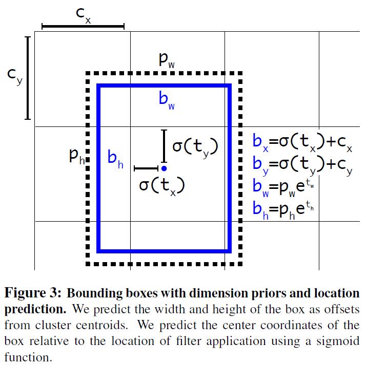

  

• Fine-grained Features: YOLO V2从$13\times 13$的feature map中预测detection，这对于large objects而言是足够的，对于small objects detection，可以从finer grained features中获益。Faster RCNN和SSD都在不同尺度的feature maps上滑窗proposal networks，来获取不同resolution的region proposal。YOLO V2采用了不同的方法来达到这种效果，即仅仅通过新增一个passthrough layer来获取earlier layer的resolution ($26\times 26$)。

  The passthrough layer concatenates the higher resolution features with the low resolution features by stacking adjacent features into different channels instead of spatial locations, similar to the identity mappings in ResNet. This turns the $26\times 26\times 512$ feature map into a $13\times 13\times 2048$ feature map, which can be concatenated with the original features. Our detector runs on top of this expanded feature map so that it has access to fine grained features. This gives a modest 1% performance increase.

• Multi-Scale Training: Instead of fixing the input image size we change the network every few iterations. Every 10 batches our network randomly chooses new image dimensions. Since our model downsamples by a factor of 32, we pull from the following multiples of $32: {320, 352, …, 608}$. Thus the smallest option is $320\times 320$ and the largest is 608×608. We resize the network to that dimension and continue training. This regime forces the network to learn to predict well across a variety of input dimensions. This means the same network can predict detections at different resolutions.

Faster

大多数detector使用了VGG作为feature extraction backbone，尽管VGG很强大，但是FLOPs太高。YOLO使用了GoogLeNet作为backbone，在YOLO V2中，作者使用了Darknet-19作为backbone。

Stronger

YOLO V2使用了一种joint training方法来训练classification和detection dataset，简而言之呢，就是说当遇到classification data时，只BP classification-specific part；当遇到detection data时，BP full architecture.

We propose a mechanism for jointly training on classification and detection data. Our method uses images labelled for detection to learn detection-specific information like bounding box coordinate prediction and objectness as well as how to classify common objects. It uses images with only class labels to expand the number of categories it can detect. During training we mix images from both detection and classification datasets. When our network sees an image labelled for detection we can backpropagate based on the full YOLOv2 loss function. When it sees a classification image we only backpropagate loss from the classificationspecific parts of the architecture.

• Hierarchical classification: 因ImageNet是Hierarchy的结构，所以为了让detector获取识别9000-category的识别能力，YOLO V2使用了一种Hierarchical classification方法。这个就不细说了，详情请参考Paper原文吧。

YOLO v3

Paper: Yolov3: An incremental improvement

YOLO v3在one-stage detector里面性能非常强大，与v1和v2相比，idea的novelty并没有什么太大的创新，更多的是借鉴了当前一些CV/DL领域的idea做了改进，本小节就来简要介绍一下YOLO v3。
主要改进如下：

1. Loss回传方面：若bbox prior没有被分配到groundtruth object，则不会引入coordinate loss和class prediction loss，而只有objectness。
2. Class prediction方面：将softmax替换为independent logistic classifier，使得其更适合multi-label classification场景。
3. 多尺度预测：在每个scale预测3个bbox，因此可以得到$N\times N\times [3\times (4+1+80)]$的tensor，来满足4个bbox offsets、1个objectness prediction，以及80个category。
4. 借鉴FPN获取更rich的feature representation：将earlier layer的feature与upsample之后的high-level features进行concatenate，来获取高层semantic meaning更强的信息，以及低层更fine-grained的信息。然后添加额外的conv layers进行进一步提纯。
5. 与YOLO v2一样，同样使用KMeans进行bbox prior的选取，一共有9个clusters：$(10\times 13), (16\times 30), (33\times 23), (30\times 61), (62\times 45), (59\times 119), (116\times 90), (156\times 198), (373\times 326)$。
6. DarkNet53 as backbone：常规套路，引入了shortcut结构。

MTCNN

Paper: Joint face detection and alignment using multitask cascaded convolutional networks

这里介绍一下人脸检测领域一个非常著名的算法——MTCNN，和通用物体检测相比，人脸检测相对来讲会容易一些。因为熟悉two-stage detection的同学应该知道，face detection可以视为一个face/non-face binary classification问题，所以binary classification的decision boundary要比multi-class classification的decision boundary更容易学得。

在MTCNN中，作者提出了一个deep cascade multi-task framework，来用一种coarse-to-fine的方法同时处理face detection和face alignment任务，此外，本文也介绍了一种online hard sample mining strategy来进一步提升性能。

MTCNN主要包括3个子网络：

• 在第一阶段，通过一个shallow CNN PNet快速生成candidate windows。
• 在第二阶段，通过一个稍微复杂的CNN RNet来reject大量non-facial candidate windows。
• 在第三阶段，通过一个更加复杂CNN ONet来进一步提纯结果，并输出5个facial landmarks。

MTCNN的pipeline如下：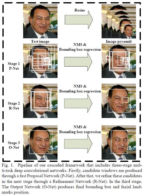

Details of MTCNN

输入图像首先被resize成不同的scale来形成image pyramid，来使得网络具备scale-invariance。然后作为下面3阶段网络的输入：

• Stage 1: 在第一阶段，PNet来得到candidate facial windows以及对应的bbox regression vectors，bbox regression对estimated bbox进行校准。然后，non-max suppression来merge highly overlapped candidates。
• Stage 2: 在Stage 1产生的candidate regions被输入到另外一个CNN——RNet，来进一步reject non-facial candidates。同时也应用bbox regression进行box校准，以及non-max suppression来merge highly overlapped candidates。
• Stage 3: 在第三阶段，ONet会输出5个facial landmarks。

Training of MTCNN

1. Face classification:
   $$
   L_i^{det}=-(y_i^{det}log(p_i) + (1-y_i^{det})(1 - log(p_i)))
   $$
2. Bounding box regression: 对于每一个candidate window，我们预测该candidate和与其最近的groundtruth box之间的offset，优化L2 Loss：
   $$
   L_i^{box}=||\hat{y}_i^{box}-y_i^{box}||_2^2
   $$
3. Facial landmark location:
   $$
   L_i^{landmark}=||\hat{y}_i^{landmark}-y_i^{landmark}||_2^2
   $$
4. Multi-source training: 因为是multi-task learning，且每个stage学习的data source都不一样(例如PNet需要face/non-face region)，所以MTCNN的整个优化目标如下：
   $$
   \mathop{min} \sum_{i=1}^N \sum_{j\in \{det, box, landmark\}}\alpha_j \beta_i^j L_i^j
   $$
5. Online hard sample mining: 在每个mini-batch里，我们对feedforwad propagation的samples按照loss进行排序，然后选择Top 70%作为hard samples，在BP的时候就只计算这些hard samples的gradients。这就意味着太容易区分的样本就直接被舍弃了。

R-FCN

Paper: R-FCN: Object Detection via Region-based Fully Convolutional Networks

这篇文章主要提出了一个Region-based Fully Convolutional Network来处理detection问题，和之前的region-based detector (例如Fast/Faster RCNN)不同，R-FCN能够做到在整张图上共享计算量，而Fast/Faster RCNN需要应用一个per-region RoI subnetwork多次，这种方式计算量就太大了。

我们知道，近些年来的一些网络结构(例如GoogLeNet/ResNet等)都是全卷积结构的，那么是否可以直接将全卷积网络直接用作detection的backbone呢？然而，这种方式在实验中发现检测精度非常低。因此，Kaiming在ResNet Paper中做detection的实验时，将RoI Pooling Layer插在两段conv layers之间，来产生deeper RoI-wise subnetwork以提高精度，但由于RoI Pooling Layer没有共享计算，所以速度上依然比较慢。

作者认为，这种不合理设计(将RoI Pooling Layer插在两段conv layers之间，来产生deeper RoI-wise subnetwork)的根源在于：image classification需要translation invariance (意思就是说无论你图像怎么平移、怎么变换，依然不会对label semantic meaning造成影响)，而object detection则需要translation variance (因为检测不仅需要object recognition，还需要bbox localisation)。

我们设想在一个图像分类网络的deeper conv layer对translation是很不敏感的，为了处理这个问题，ResNet Paper中在conv layer中插入了RoI pooling layer，这种region-specific operation破坏了原来分类网络中的translation invariance，因此post-RoI conv layer在across different region evaluation时就不再是translation-invariant了。但是因为引入了一些region-wise layers，所以速度上肯定就自然慢了一些。

本文提出了R-FCN，来将translation variance引入到网络中来。通过一系列特殊的conv layer来构造position-sensitive score maps来作为FCN的输出。每个score map都encode了relative spatial position information (例如某个object的左边)。在FCN的顶层，作者额外添加了position-sensitive RoI pooling layer来从这些score maps中得到spatial information，并且没有引入任何额外的weight conv/fc layers。所有learnable layers都是conv layers，并且在整张图上共享，因此encode了detection所需的spatial information。

Delve into RFCN

Overview

先来看一下RFCN的大致流程：给定一系列region proposals (RoIs)，RFCN来将这些region proposals进行分类。FRCN中所有layers都是conv layer，并且是在entire image上进行计算的。最后一个conv layer对每一个category都产生一系列$k^2$个position-sensitive score maps。因此就得到了$k^2(C+1)$-channel的输出，其中$C+1$代表$C$个categories + $1$个background。$k^2$个score maps对应的$k\times k$的spatial grid描述了relative positions。

For example, with $k\times k = 3\times 3,$ the 9 score maps encode the cases of {top-left, top-center, top-right, ..., bottom-right} of an object category.

RFCN以positive-sensitive RoI pooling layer结尾，该pooling layer将最后一个conv layer的输出进行综合，并对每个RoI输出scores。

Note：our position-sensitive RoI layer conducts selective pooling, and each of the $k\times k$ bin aggregates responses from only one score map out of the bank of $k\times k$ score maps. With end-to-end training, this RoI layer shepherds the last convolutional layer to learn specialized position-sensitive score maps.。

Position-sensitive score maps & Position-sensitive RoI pooling

为了将position information encode到RoI，我们将每个RoI rectangle划分到$k\times k$个bin (对于size为$w\times h$的RoI，每个bin的size是$\frac{w}{k}\times \frac{h}{k}$)。在RFCN中，最后一个conv layer用来对每个category产生$k^2$个score maps。在第$(i,j)$-th 个bin中，我们定义position-sensitive RoI pooling 来仅仅在第$(i,j)$-th 个score map上进行pool操作。
$$
r_c(i,j|\Theta)=\sum_{(x,y)\in bin(i,j)}z_{i,j,c} (x + x_0, y + y_0|\Theta)/n
$$

$r_c(i,j)$是对应第$c$个category、第$(i,j)$个bin的pooled response，$z_{i,j,c}$是$k^2(C+1)$之外的score map，$(x_0, y_0)$代表RoI中top-left corner (因为我们之前提到过这是relative spatial information)，$n$代表bin中的像素点。第$(i,j)$个bin横跨$\lfloor i \frac{w}{k}\rfloor \leq x < \lceil (i+1)\frac{w}{k}\rceil$、$\lfloor j \frac{h}{k}\rfloor \leq y < \lceil (j+1)\frac{h}{k}\rceil$。

接下来，$k^2$个position-sensitive score在RoI上进行voting，本文简单粗暴地使用averaging来voting，然后对于每个RoI产生$(C+1)$-d的vector：$r_c(\Theta)=\sum_{i,j} r_c(i,j|\Theta)$，然后就是进softmax layer分类。

The concept of position-sensitive score maps is partially inspired by [3] that develops FCNs for instance-level semantic segmentation. We further introduce the position-sensitive RoI pooling layer that shepherds learning of the score maps for object detection. There is no learnable layer after the RoI layer, enabling nearly cost-free region-wise computation and speeding up both training and inference.

Training

训练过程和Fast/Faster RCNN类似：

With pre-computed region proposals, it is easy to end-to-end train the R-FCN architecture.
Following [7], our loss function defined on each RoI is the summation of the cross-entropy loss and the box regression loss: $L(s, t_{x,y,w,h})=L_{cls}(s_{c^{\star}}) + \lambda [c^{\star} > 0]L_{reg}(t,t^{\star})$. Here $c^{\star}$ is the RoI’s ground-truth label ($c^{\star}=0$ means background). $L_{cls}(s_{c^{\star}})=-log(s_{c^{\star}})$ is the cross-entropy loss for classification, $L_{reg}$ is the bounding box regression loss as defined in [7], and $t^{\star}$ represents the ground truth box. $[c^{\star} > 0]$ is an indicator which equals to 1 if the argument is true and 0 otherwise. We set the balance weight $\lambda = 1$ as in [7]. We define positive examples as the RoIs that have intersection-over-union (IoU) overlap with a ground-truth box of at least 0.5, and negative otherwise.

It is easy for our method to adopt online hard example mining (OHEM) [23] during training. Our negligible per-RoI computation enables nearly cost-free example mining. Assuming $N$ proposals per image, in the forward pass, we evaluate the loss of all $N$ proposals. Then we sort all RoIs (positive and negative) by loss and select B RoIs that have the highest loss. Backpropagation [12] is performed based on the selected examples. Because our per-RoI computation is negligible, the forward time is nearly not affected by $N$, in contrast to OHEM Fast R-CNN in [23] that may double training time.

FPN

Paper: Feature Pyramid Networks for Object Detection

最近在写硕士毕业论文，魔改了一个网络叫作Cascaded Feature Pyramid Network (CFPNet)，提到feature pyramid，那就不得不提FPN了。熟悉detection的同学都知道，detection领域一个导致bbox框不准的原因就是scale variance。而解决multi-scale的方法常见的有Image Pyramid和Feature Pyramid，其中，Image Pyramid在MTCNN中用到过；Feature Pyramid在之前非deep的传统方法也是很常用的(其实SSD也一定程度上用到了multi-scale training)。这样虽然会提升精度，但是计算量也大大增加了，聪明的读者一点立马就想到了：既然CNN本身的feature map就是from coarse to fine + hierarchical multi-scale的结构，那可不可以直接取CNN的feature map来构造feature pyramid呢？没错！这就是FPN的main idea！

构造Pyramid大致有一下几种常见的方法：

The principle advantage of featurizing each level of an image pyramid is that it produces a multi-scale feature representation in which all levels are semantically strong, including the high-resolution levels.

本文提出的feature pyramid构造方式如下：up是只在finest level上做prediction，bottom是在每个level上都做prediction。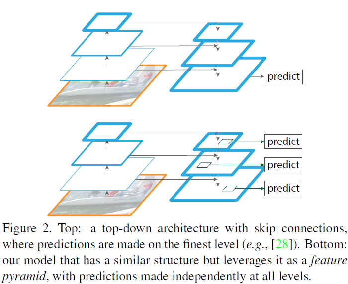

Feature Pyramid Networks

FPN可以接受任意尺寸的single-scale image作为输入，然后以全卷积的方式输出对应成比例multi-scale的feature map。该步骤与具体的backbone network无关。FPN用到了bottom-up pathway，top-down pathway和lateral connection3种结构来构造feature pyramid。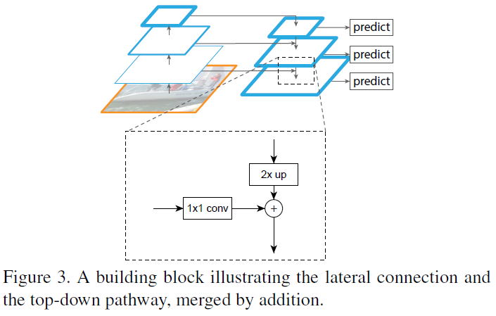

Bottom-up pathway

所谓bottom-up pathway，即从底层到高层，就是在网络中走了一遍feedforwad，然后产生了一系列multi-scale feature map hierarchy (scaling step=2 in ResNet)。熟悉ResNet的同学们都知道，ResNet中引入了skip connection来辅助信息流通，ResNet中的shortcut实际上就是Element-wise addition，也就是说每个residual block的output feature map size都是相同的。因此在FPN中作者定义这样的layer为stage，并且在每个stage中都定义一个pyramid level。作者选择每个stage最后一层的output来作为reference set，用来构造pyramid (因为每个stage中deepest layer有着strongest feature)。

Specifically, for ResNets [16] we use the feature activations output by each stage’s last residual block. We denote the output of these last residual blocks as {C2, C3, C4, C5} for conv2, conv3, conv4, and conv5 outputs, and note that they have strides of {4, 8, 16, 32} pixels with respect to the input image. We do not include conv1 into the pyramid due to its large memory footprint.

Top-down pathway and lateral connections

所谓top-down pathway，即从高层到底层，了解CNN的同学都知道，high layer包含更丰富的semantic meaning，而low layer包含更多的fine-grained details。但是high layer经过了多次的pooling，所以size自然变得更小了，所以我们就需要首先对其进行upsampling操作。然后通过lateral connection和bottom-up pathway一起enhance得到更强的representation。通过lateral connection连接的feature map size都是一致的，bottom-up的feature包含的semantic meaning比较少，但是细节信息比较多，所以非常适合localisation任务(因为没有经历那么多pooling layer丢失spatial information)。

With a coarser-resolution feature map, we upsample the spatial resolution by a factor of 2 (using nearest neighbor upsampling for simplicity). The upsampling pled map is then merged with the corresponding bottom-up map (which undergoes a 1×1 convolutional layer to reduce channel dimensions) by element-wise addition. This process is iterated until the finest resolution map is generated.

To start the iteration, we simply attach a 1×1 convolutional layer on C5 to produce the coarsest resolution map. Finally, we append a 3×3 convolution on each merged map to generate the final feature map, which is to reduce the aliasing effect of upsampling. This final set of feature maps is called {P2, P3, P4, P5}, corresponding to {C2, C3, C4, C5} that are respectively of the same spatial sizes.

因为这些pyramids的所有level用的都是shared classifier/regressor，所以我们将feature dimension固定($d=256$)。

Feature Pyramid Networks for RPN

熟悉Faster RCNN的同学自然对RPN不会陌生了，RPN实际上就是个小的fully convolutional network，以sliding window的方式在feature map上滑动来产生region proposals。在最初的RPN设计中，用了一个小型的subnetwork来在dense $3\times 3$ sliding windows上做object classification和bbox regression。

既然RPN是个fixed window size的sliding window detector，所以再scanning pyramid level的feature map之后，能够提升其对scale variance的鲁棒性。

This is realized by a $3\times 3$ conv layer followed by two sibling $1\times 1$ conv for classification and regression.

这里我们称之为network head，object/non-object和bbox regression target的定义取决于一系列reference boxes(我们称之为anchors)。这些anchors包含了pre-defined scales and aspect ratios来cover各种size和scale的object，以保证high recall。

作者将RPN中的single-scale feature map替换为FPN，原来的结构保持不变，即依然是一个$3\times 3$ conv layer再接2个sibling $1\times 1$ conv 做object classification和bbox regression。只不过这个head接在了feature pyramid上。(换言之，输送到multi-task loss的feature是feature pyramid而非原来的single scale)。

Because the head slides densely over all locations in all pyramid levels, it is not necessary to have multi-scale anchors on a specific level. Instead, we assign anchors of a single scale to each level. Formally, we define the anchors to have areas of {322, 642, 1282, 2562, 5122} pixels on {P2, P3, P4, P5, P6} respectively.1 As in [29] we also use anchors of multiple aspect ratios {1:2, 1:1, 2:1} at each level. So in total there are 15 anchors over the pyramid.

作者注意到，head中的参数在所有feature pyramid levels都是共享的，同时对比了不共享的实验，发现不共享的accuracy也是一样的。

The good performance of sharing parameters indicates that all levels of our pyramid share similar semantic levels. This advantage is analogous to that of using a featurized image pyramid, where a common head classifier can be applied to features computed at any image scale.

Feature Pyramid Networks for Fast RCNN

Fast RCNN通常运行在single-scale feature map上，为了将FPN用在Fast RCNN中，我们需要分配不同scale的RoI对应的pyramid levels。

We view our feature pyramid as if it were produced from an image pyramid. Thus we can adapt the assignment strategy of region-based detectors in the case when they are run on image pyramids. Formally, we assign an RoI of width $w$ and height $h$ (on the input image to the network) to the level $P_k$ of our feature pyramid by:
$$
k=\lfloor k_0 + log_2(\sqrt{wh}/224)\rfloor
$$

224是ImageNet pretraining size，$k_0$是RoI($w\times h=224^2$)应该被映射到的target level，实验中设置$k_0=4$。

Intuitively, Eqn. (1) means that if the RoI’s scale becomes smaller (say,1/2 of 224), it should be mapped into a finer-resolution level (say, $k=3$).

DetNet

Paper: DetNet: A Backbone network for Object Detection

Deep Learning在Detection取得了越来越多的成果，但是我们通常将分类网络直接拿过来作为detection的backbone，这样的好处是可以直接利用ImageNet pretrained weights。但是毕竟Classification和Detection是不一样的，detection除了要做object recognition之外，还需要给出bbox location。直接使用classification network作为detection的backbone有以下问题：

• 需要额外的stage来处理multi-scale的object (例如FPN)
• deep classification network中包含了许多的pooling layer，随着网络层数的加深，receptive fields是变大了，但是spatial information越来越少了。所以用于classification的网络结构未必是detection中最优的。

在DetNet中，作者专门设计了additional stage来处理variant scales，但和分类网络不同的是：尽管新增了additional stage，feature map的spatial resolution依然保持不变。此外，为了保证efficiency，DetNet使用了dilated bottleneck structure，这样既可以保证high resolution的feature map，又可以保证large receptive fields。

DetNet: A Backbone network for Object Detection

Motivation

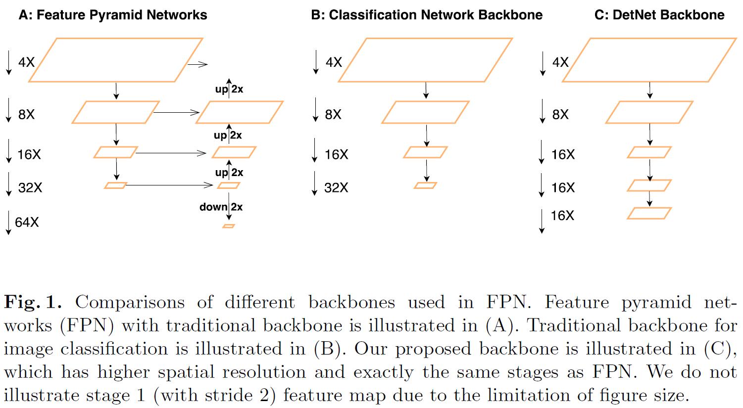
• The number of network stages is different. 典型的classification network包含5个stage (如上图B所示)，每个stage经历$2\times$ pooling或stride=2的conv，因此spatial size被下采样了$2^5=32\times$ 次。和classification network不同，FPN通常采用了更多的stage。
• Weak visibility of large objects. 包含rich semantic information的feature map相对于input image进行了$32\times$ donw-sampling，这样会得到large receptive fields，有利于classification。但是过多的down-sampling带来了spatial information lose，这样会降低detection的性能。
• Invisibility of small objects. 随着context information被encode进来、feature map的spatial resolution越来越低，small object就越来越难被检测到。FPN采取的方法是在shallower layer中预测小物体。但是shallow layer包含的semantic meaning太少了，所以很难预测该object的类别。因此detector必须encode high-level representation来加强其分类能力。

和传统detection backbone相比，DetNet有如下优点：

• DetNet和其他backbone network有几乎一样数量的stage，因此extra stage可以直接在ImageNet上pretrain。
• 受益于最后一个stage的high resolution feature map，DetNet在检测小物体方面更有优势。

The detail design of our DetNet59 is illustrated as follows:

• We introduce the extra stages, e.g., P6, in the backbone which will be later utilized for object detection as in FPN. Meanwhile, we fix the spatial resolution as $16\times$ downsampling even after stage 4.
• Since the spatial size is xed after stage 4, in order to introduce a new stage, we employ a dilated [29,30,31] bottleneck with $1\times 1$ convolution projection (Fig. 2B) in the begining of the each stage. We nd the model in Fig. 2B is important for multi-stage detectors like FPN.
• We apply bottleneck with dilation as a basic network block to efficiently enlarge the receptive led. Since dilated convolution is still time consuming, our stage 5 and stage 6 keep the same channels as stage 4 (256 input channels for bottleneck block). This is dierent from traditional backbone design, which will double channels in a later stage.

网络结构示意图如下：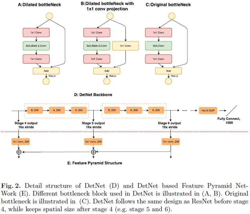

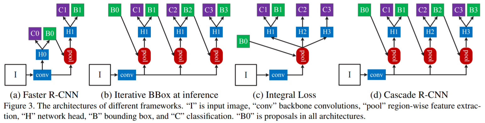
Cascade RCNN

Paper: Cascade R-CNN: Delving into High Quality Object Detection

熟悉detection的同学都应该知道，现如今主流的two-stage detection framework是基于RCNN改进而来的，即将detection问题转化为classification问题。而在classification的时候，我们通常会根据IOU的阈值来设定positive samples与negative samples。那么问题来了，若IOU卡得越严，positive samples的数量就会大幅度降低，而negative samples的数量则会大幅增加。因此会引发overfitting问题，并且DNN本身也无法得到最优解。通常情况下我们设定IOU threshold为0.5，但该阈值毕竟比较宽松，带来的缺陷就是很容易产生过多的FP(False Positive)。

Cascade RCNN就是为了解决这些问题，cascade一词，意思为在训练过程中，通过逐渐增加IOU threshold的值来对FP识别得更好，以及通过resampling来保证sample size平衡。此外，与MTCNN中cascade一词类似，Cascade RCNN也是trained stage-by-stage，并且假定前一个stage中detector的输出能为下一个stage detector的training set提供很好的distribution，因此也是类似的“逐步提纯”的idea。

在Cascade RCNN中，作者将一个hypotheses的quality定义为其与groundtruth bbox的IOU，并且将quality of detector定义为用来训练模型的IOU阈值u。每个threshold下的detector只负责自己学到当前最佳，也就是说在某个IOU threshold下最佳的detector并不一定能保证在其他IOU threshold下的最佳。

Fundamentation of Object Detection

Cascade RCNN延续了Faster RCNN的设计风格，即head $H_0$生成region proposal(即preliminary detection hypotheses)；head $H_1$同时进行object classification + bbox regression。

为了使得regression对scale/location更加invariant，$L_{loc}$通常在distance vector $\Delta=(\delta_x, \delta_y, \delta_w, \delta_h)$上进行操作。
$$
\delta_x = (g_x-b_x)/b_w
$$

$$
\delta_y = (g_y-b_y)/b_h
$$

$$
\delta_w = log(g_w/b_w)
$$

$$
\delta_h = log(g_h/b_h)
$$
其中$g$代表groundtruth bbox，$b$代表candidate bbox。

大多数情况下，bbox都是画得比较准的，也就是说bbox regression只会对candidate bbox $b$做细微的调整，因此regression loss会比classification loss小很多。为了提升multi-task learning的有效性，$\Delta$通常被mean和variance归一化，即$\delta_x$被替换为：
$$
\delta_x^{‘}=(\delta_x-\mu_x)/\sigma_x
$$

近期的一些research work认为单个bbox regression无法实现对localization的精准定位，因此，这些工作将多个regressor串联起来作为post-processing step:
$$
f^{‘}(x,b)=f\circ f\circ \cdots \circ f(x, b)
$$
这种方法称为Interative BBox Regression。

前面提到过，在将bbox patch进行classification时，通常根据IOU threshold $u$ 来划分positive/negative samples，若 $u$ 太大，则positive samples数量比较少；若 $u$ 太小，positive samples的diversity和richness比较丰富，但detector却无法reject close FP samples。

Delve into Cascade RCNN

Cascaded BBox Regression

前面已经提到过，用一个regressor试图为每一个level提供良好的bbox regression result是非常困难的事情。在Cascade RCNN中被建模为cascade regression problem:
$$
f(x,b)=f_T\circ f_{T-1}\circ \cdots \circ f_1(x,b)
$$
其中，第 $t$ 个stage 的 regressor $f_t$ 是在上一个stage 输出的 $\{b^t\}$ 上进行优化，而非初始集合 $\{b^1\}$，即为Cascade一词的含义。

和Iterative BBox Regression相比，Cascade BBox Regression主要有如下几点不同：

1. Iterative BBox Regression是一个post-processing procedure，主要用来提升BBox；而Cascade BBox Regression是一个resampling procedure，主要为了改变不同stage下的hypotheses distribution。
2. Cascade BBox Regression在training和inference阶段都使用。
3. $\{f_T,f_{T-1},\cdots,f_1\}$在不同stage的resampled distribution下优化，而不是对最初的distribution $\{b^1\}$优化。

Cascaded Detection

在原文的实现中，将后续stage的positive samples设定为一个恒定的值，来保证当IOU threshold增加时，training set依然有足够的positive samples。

在第 $t$ 个stage、IOU threshold为 $u^t$ 的情况下，loss定义为：
$$
L(x^t,g)=L_{cls}(h_t(x^t), y^t) + \lambda [y^t\geq 1]L_{loc}(f_t(x^t, b^t), g)
$$
其中$b^t=f_{t-1}(x^{t-1},b^{t-1})$。

Focal Loss

Paper: Focal Loss for Dense Object Detection

Focal Loss是Kaiming He团队发表在ICCV’17上的工作，这篇paper主要contribution如下：

1. 分析了one-stage在精度上不如two-stage detector的原因在于严重的正负样本(background VS objects)不均衡，Focal Loss通过down-weight easy examples的gradient来使模型在学习中更加地关注hard examples。
2. 借助Focal Loss，设计了一个非常强大的one-stage detector——RetinaNet。

下面来进行详细讲解，数据不平衡问题是Machine Learning领域一个非常常见且非常头疼的问题(有空我会将Leanring from Imbalanced Data写成一个专题，此处就先大致介绍一下paper中的related work吧)，imbalanced dataset会让模型更偏向数量多的类别，从而overwhelm整体性能。

Imbalanced dataset learning主要有如下两点问题：

1. Training是非常inefficient的，因为大多数都是easy negative samples，模型学不到什么真正有用的signal和精确的decision boundary。
2. 模型会更偏向数量多的类，如前面我们提到的。

值得一提的是，Focal Loss和Huber Loss之间的区别：

• Huber Loss通过down-weight hard samples的loss来减少outliers的contribution。
• 而Focal Loss则恰恰相反，它通过down-weight easy samples的loss来处理数据不平衡问题，即尽管easy samples的数量很多，但是它们对total loss的contribution就被抑制了。

总而言之，Focal Loss的主体思路和Huber Loss恰好相反，它更多地关注a sparse set of hard examples。

Delve into Focal Loss

在介绍Foal Loss之前，先来分析CrossEntropy Loss(CE)：
$$
CE(p,y)=
\begin{cases}
-log(p) & \text{if}\quad y=1\\
-log(1-p) & otherwise
\end{cases}
$$
令：
$$
p_t=
\begin{cases}
p & \text{if}\quad y=1\\
1-p & otherwise
\end{cases}
$$
可得：
$$
CE(p,y)=CE(p_t)=-log(p_t)
$$
但是CE有什么问题呢？通过可视化gt labels的probability可以发现：即便是对于非常容易分类的easy examples，依然会引入不小的loss(如下图所示)，而这些samples会影响数量较少对应类的学习。

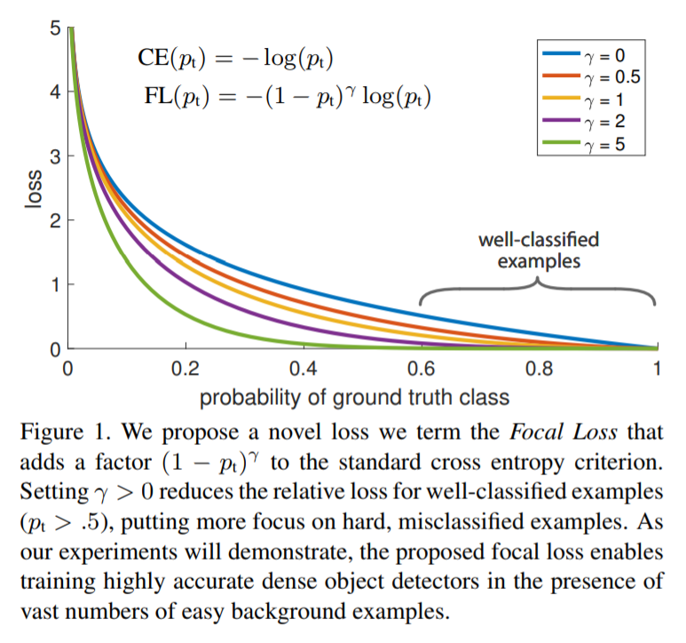
常见的处理方法是weighted cross entropy，即引入一个权重系数$\alpha\in [0,1]$，对positive/negative分别分配$\alpha$与$1-\alpha$。在实践中，$\alpha$通常设置为对应类别frequency的倒数，或通过cross validation进行选取，$\alpha$-weighted CE可表示为：
$$
CE(p_t)=-\alpha_t log(p_t)
$$

Focal Loss定义如下：
$$
FL(p_t)=-(1-p_t)^{\gamma}log(p_t)
$$
Focal Loss有如下性质：

1. 当一个sample被错误分类并且$p_t$很小时，调整系数$(1-p_t)^{\gamma}$接近1，因此loss几乎不受影响；而当$p_t$很大时，调整系数接近0，因此easy-classified samples的loss就被抑制了。
2. $\gamma$可以平滑地调整easy samples被down-weighted的节奏。$\gamma=0$时，$FL=CE$；$\gamma$递增，调整系数的作用也递增，促使模型更多地关注hard samples、远离easy samples。实验中通常设置$\gamma=2$。

$\alpha$-weighted Focal Loss即为：
$$
FL(p_t)=-\alpha_t (1-p_t)^{\gamma}log (p_t)
$$

与Online Hard Example Mining的关系：OHEM通过使用high-loss examples来构造minibatch，和Focal Loss类似，OHEM也是更关注misclassified examples；但与Focal Loss不同的是，OEHM完全丢弃了easy samples。

Repulsion Loss

Paper: Repulsion loss: Detecting pedestrians in a crowd

熟悉detection的同学应该都知道，detection场景有一个非常棘手的问题就是密集、目标之间重叠严重的检测。Repulsion Loss就是为了一定程度上解决以上问题，Repulsion Loss是发表在CVPR’18上的paper，在行人检测和常规目标检测都取得了非常好的效果。Repulsion Loss是针对bbox regression步骤中的loss改进，主要idea就是让predicted bbox与gt bbox尽可能接近，同时和其他object尽可能远离。

Detection中的occlusion可分为两种：

1. inter-class occlusion: 不同category目标之间的遮挡
2. intra-class occlusion: 被相同category目标相互之间的遮挡，也称为crowd occlusion，更多时候，intra-class occlusion是更棘手的，因为大多数场景下，相同类别的samples appearance总是比不同类别的samples appearance更相似

传统的bbox regression loss(例如$L_2$ Loss, Smooth $L_1$ Loss)只会push让predicted bbox和target gt bbox更接近；而Repulsion Loss不仅可以让proposal bbox与gt bbox更接近，还能让该proposal bbox与其他gt bbox更远离，以及与其他非该类的proposal bbox也更远离。

本文提出了两种Repulsion Loss：RepGT Loss与RepBox Loss。

• RepGT Loss对shift到其他gt bbox的predicted bbox进行惩罚；RepGT Loss对于减少FP非常有用
• RepBox Loss则需要每个predicted bbox都与其他不同target对应predicted bbox尽可能远离，这样可以使得detection results对NMS更加不敏感。

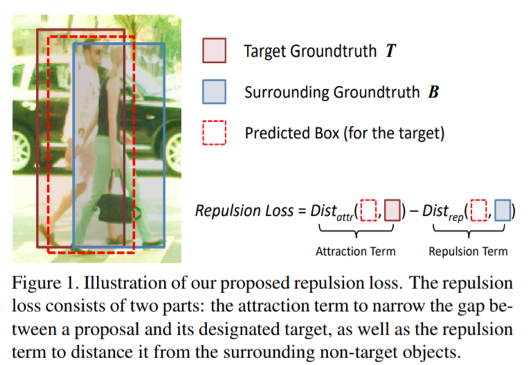
Delve into Repulsion Loss

Repulsion Loss主要由以下3部分组成：
$$
L=L_{Attr} + \alpha\times L_{RepGT} + \beta\times L_{RepBox}
$$
其中，$L_{Attr}$代表attraction term，作用是让predicted bbox尽可能接近gt bbox；$L_{RepGT}$作用是让某个predicted bbox与它周围的gt bbox远离；$L_{RepBox}$作用是某个predicted bbox与其他predicted bbox远离。

定义$P=\{l_P,t_P,w_P,h_P\}$代表proposal bbox，$G=\{l_G,t_G,w_G,h_G\}$代表gt bbox。$\mathcal{P}_{+}=\{P\}$代表所有positive proposals ($IOU\geq 0.5$) 的集合，$\mathcal{G}=\{G\}$代表一张图中所有的gt bbox。

• Attraction Term可以定义为：
  $$
  L_{Attr}=\frac{\sum_{P\in \mathcal{P}_{+}} Smooth_{L1}(B^P,G_{Attr}^P)}{|\mathcal{P}_{+}|}
  $$

• RepGT Loss的作用是让proposal bbox与其周围其他的 (非本proposal对应的gt) gt bbox远离。故RepGT objects可定义为：
  $$
  G_{Rep}^P=\mathop{argmax} \limits_{G\in \mathcal{G}\smallsetminus\{G_{Attr}^P\}} IoU(G, P)
  $$

RepGT Loss为对$B^P$与$G_{Rep}^P$之间overlap的惩罚，其中overlap为$B^P$与$G_{Rep}^P$之间之间的IoG (Intersection over Groundtruth)：
$$
IoG(B,G)\triangleq \frac{area(B\bigcap G)}{area(G)}\in [0,1]
$$

因此，RepGT Loss为：
$$
L_{RepGT}=\frac{\sum_{P\in \mathcal{P}_{+}}Smooth_{ln}(IoG(B^P,G_{Rep}^P))}{|\mathcal{P}_{+}|}
$$

其中，
$$
Smooth_{ln}=\begin{cases}
-ln(1-x) & x\leq \sigma\\
\frac{x-\sigma}{1-\sigma}-ln(1-\sigma) & x> \sigma
\end{cases}
$$
$\sigma$越小，loss对outliers越不敏感。

• RepBox Loss作用是让proposal bbox与其他不同target的proposal bbox更远离。将proposal set $\mathcal{P}_{+}$划分为多个不相交的子集: $\mathcal{P}_{+}=\mathcal{P}_{1}\bigcap \mathcal{P}_{2}\bigcap \cdots \bigcap \mathcal{P}_{|\mathcal{G}|}$。因此对于任意两个randomly sampled proposal $P_i\in \mathcal{P}_i$与$P_j\in \mathcal{P}_j$，我们希望predicted bbox $B^{P_i}$与$B^{P_j}$之间的overlap尽可能小。因此，RepBox Loss可定义为：
  $$
  L_{RepBox}=\frac{\sum_{i\neq j}Smooth_{ln}(IoU(B^{P_i},B^{P_j}))}{\sum_{i\neq j}\mathbb{1}[IoU(B^{P_i},B^{P_j})>0] + \epsilon}
  $$

在Repulsion Term中选择IoU或IoG，而非Smooth $L_1$作为distance metric的原因在于：IoU/IoG在$[0,1]$区间内，而Smooth $L_1$是boundless的。若在RepGT Loss中使用Smooth $L_1$，则会使得predicted bbox与repulsion gt bbox尽可能地远离。而IoG只会让predicted bbox与repulsion gt bbox之间的overlap最小化。

此外，在RepGT Loss中采用IoG而非IoU的原因在于：若使用IoU-based loss，则bbox regressor会通过简单扩大bbox size来增大分母$area(B^P\bigcup G_{Rep}^P)$，从而达到最小化IoU loss的目的。而IoG的分母是一个常数，因此可以让bbox regressor直接最小化$area(B^P\bigcap G_{Rep}^P)$。

Libra RCNN

Paper: Libra R-CNN: Towards Balanced Learning for Object Detection

Libra RCNN是发表在CVPR’19上的文章，我在商品检测项目中也用到了这个算法，效果的确是非常nice，而且idea也非常简单易懂。本小节就来对这个工作进行介绍。

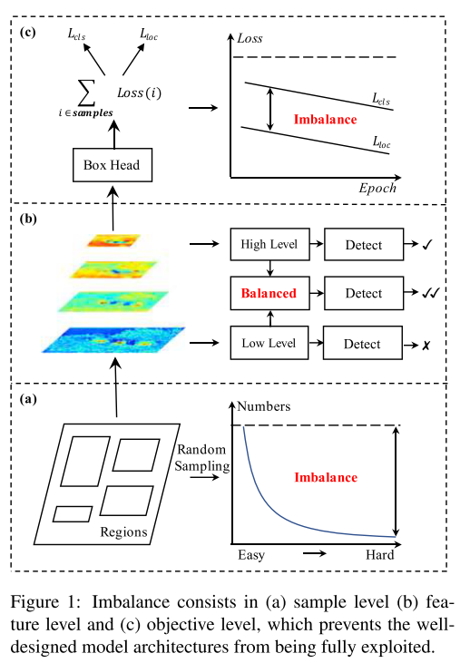
从paper title也可以知道，Libra RCNN是属于RCNN系列的two-stage detector，并且着重点在于balanced learning，该算法主要从以下3点来解决imbalanced learning问题：

• Sample level: 提出了IoU-balanced sampling
• Feature level: 提出了balanced feature pyramid
• Loss level: 提出了balanced L1 loss

过去几年见证了Deep Learning在Object Detection领域的飞速发展，从最初的RCNN到本文的Libra RCNN，其关键性因素主要有如下3点：

1. whether the selected region samples are representative
2. whether the extracted visual features are fully utilized
3. whether the designed objective function is optimal

作者发现，在上述3点均存在着imbalance问题，而这些imbalance problem会影响模型的performance。既然发现问题是为了解决问题，而这3点分别对应了sample level、feature level以及loss level的imbalance problem。

Methodology

IoU-balanced Sampling

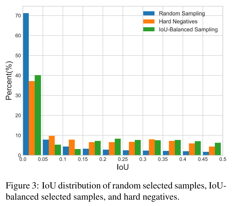
为了解决sample level的imbalance问题，作者提出了一种新的hard mining method——IoU-balanced Sampling:
若要从$M$个candidate中选出$N$个 negative samples，那么random sampling的概率为$p=\frac{N}{M}$。为了提高negative samples被select的概率，首先根据IOU将sampling interval平均划分成$K$个bin，在每个bin内部negative samples都是evenly distributed。所以在IOU-balanced sampling下，selected probability为：
$$
p_k = \frac{N}{K}\times \frac{1}{M_k} k\in [0, K)
$$
where $M_k$ is the number of sampling candidates in the corresponding interval denoted by $k$. $K$ is set to 3 by default in our experiments.

下图显示，采用了IOU-balanced sampling的方法，比randomly sampling选取的negative samples更接近真实的distribution。

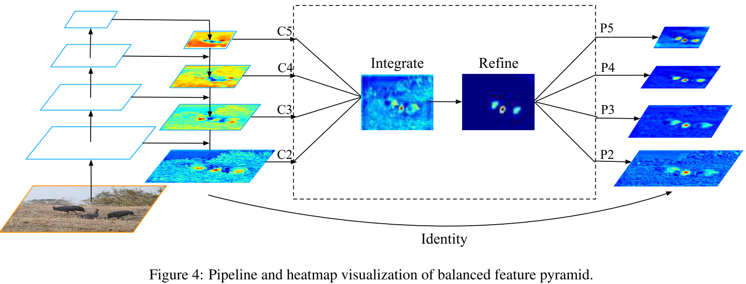
Balanced Feature Pyramid

与FPN等通过lateral path来融合multi-level feature不同，Libra RCNN是通过使用same deeply integrated balanced semantic features来增强multi-level features。该步骤主要包含rescaling, integrating, refining and strengthening 4个步骤(如下图所示)。因为步骤非常简单，也很好理解，这里就直接引用一下原文吧，不做讲解了。

• Obtaining balanced semantic features

  Features at resolution level $l$ are denoted as $C_l$. The number of multi-level features is denoted as $L$. The indexes of involved lowest and highest levels are denoted as $l_{min}$ and $l_{max}$. In Figure 4, $C_2$ has the highest resolution. To integrate multi-level features and preserve their semantic hierarchy at the same time, we first resize the multi-level features $\{C_2, C_3, C_4, C_5\}$ to an intermediate size, i.e., the same size as $C_4$, with interpolation and max-pooling respectively. Once the features are rescaled, the balanced semantic features are obtained by simple averaging as:
  $$
  C=\frac{1}{L}\sum_{l=l_{min}}^{l_{max}}C_l
  $$

  The obtained features are then rescaled using the same but reverse procedure to strengthen the original features. Each resolution obtains equal information from others in this procedure. Note that this procedure does not contain any pa- rameter. We observe improvement with this nonparametric method, proving the effectiveness of the information flow.

• Refining balanced semantic features

  作者采用了Gaussian non-local attention来enhance balanced semantic feature。

Balanced L1 Loss Classification

现在的two-stage detector几乎都是在RCNN/Faster RCNN的改进，Faster RCNN的Loss如下：
$$
L_{p,u,t^u,v}=L_{cls}(p,u) + \lambda[u\geq 1]L_{loc}(t^u,v)
$$

$L_{p,u,t^u,v}$是个典型的multi-task loss，因此调整$\lambda$是个很头疼的问题。而由于regression loss unbound的特性，直接提高regression loss的权重会使得模型对outliers十分敏感。针对这个问题，作者提出了Balanced $L_1$ Loss。

These outliers, which can be regarded as hard samples, will produce excessively large gradients that are harmful to the training process. The inliers, which can be regarded as the easy samples, contribute little gradient to the overall gradients compared with the outliers.

Balanced $L_1$ loss is derived from the conventional smooth $L_1$ loss, in which an inflection point is set to separate inliers from outliners, and clip the large gradients produced by outliers with a maximum value of 1.0.

Balanced $L_1$ Loss的目的就是为了提升crucial regression gradients(例如inliers，即accurate samples)，从而让regression loss与classification loss更加balance。
$$
L_{loc}=\sum_{i\in \{x,y,w,h\}} L_b (t_i^u-v_i)
$$
其对应的gradients满足:
$$
\frac{\partial L_{loc}}{\partial w}\propto \frac{\partial L_b}{\partial t_i^u}\propto \frac{\partial L_b}{\partial x}
$$
Gradient formulation如下：
$$
\frac{\partial L_b}{\partial x}=\begin{cases}
\alpha ln(b|x|+1) & if |x|<1\\
\gamma & otherwise
\end{cases}
$$
$\alpha$越小，inliers的gradient越大，但outliers的gradient未受影响。此外，$\gamma$也可用来调整regression error的upper bound，从而使得object function更好地balance classification/regression task。

Balanced $L_1$ Loss定义如下：
$$
L_b(x)\begin{cases}
\frac{\alpha}{b}(b|x|+1)ln(b|x|+1)-\alpha |x| & if |x|<1\\
\gamma |x| + C & otherwise
\end{cases}
$$
其中，$\gamma$, $\alpha$, $b$满足：
$$
\alpha ln(b+1)=\gamma
$$

Reference

1. Girshick, Ross, et al. “Rich feature hierarchies for accurate object detection and semantic segmentation.” Proceedings of the IEEE conference on computer vision and pattern recognition. 2014.
2. He, Kaiming, et al. “Spatial pyramid pooling in deep convolutional networks for visual recognition.” European conference on computer vision. Springer, Cham, 2014.
3. Girshick, Ross. “Fast r-cnn.” Proceedings of the IEEE international conference on computer vision. 2015.
4. Ren, Shaoqing, et al. “Faster r-cnn: Towards real-time object detection with region proposal networks.” Advances in neural information processing systems. 2015.
5. Liu, W., Anguelov, D., Erhan, D., Szegedy, C., Reed, S., Fu, C. Y., & Berg, A. C. (2016, October). Ssd: Single shot multibox detector. In European conference on computer vision (pp. 21-37). Springer, Cham.
6. Redmon, Joseph, et al. “You only look once: Unified, real-time object detection.” Proceedings of the IEEE conference on computer vision and pattern recognition. 2016.
7. Li Z, Peng C, Yu G, et al. Light-head r-cnn: In defense of two-stage object detector[J]. arXiv preprint arXiv:1711.07264, 2017.
8. Lin, Tsung-Yi, et al. “Feature Pyramid Networks for Object Detection.” CVPR. Vol. 1. No. 2. 2017.
9. Redmon, Joseph, and Ali Farhadi. “YOLO9000: Better, Faster, Stronger.” 2017 IEEE Conference on Computer Vision and Pattern Recognition (CVPR). IEEE, 2017.
10. Redmon, Joseph, and Ali Farhadi. “Yolov3: An incremental improvement.” arXiv preprint arXiv:1804.02767 (2018).
11. Zhang, Kaipeng, et al. “Joint face detection and alignment using multitask cascaded convolutional networks.” IEEE Signal Processing Letters 23.10 (2016): 1499-1503.
12. Li, Zeming, et al. “DetNet: A Backbone network for Object Detection.” arXiv preprint arXiv:1804.06215 (2018).
13. Dai, Jifeng, et al. “R-fcn: Object detection via region-based fully convolutional networks.” Advances in neural information processing systems. 2016.
14. Cai, Zhaowei, and Nuno Vasconcelos. “Cascade r-cnn: Delving into high quality object detection.” Proceedings of the IEEE Conference on Computer Vision and Pattern Recognition. 2018.
15. Lin, Tsung-Yi, et al. “Focal loss for dense object detection.” Proceedings of the IEEE international conference on computer vision. 2017.
16. Wang, Xinlong, et al. “Repulsion loss: Detecting pedestrians in a crowd.” Proceedings of the IEEE Conference on Computer Vision and Pattern Recognition. 2018.
17. Pang, Jiangmiao, et al. “Libra r-cnn: Towards balanced learning for object detection.” Proceedings of the IEEE Conference on Computer Vision and Pattern Recognition. 2019.