[ML] Loss Function in ML

Introduction

Loss Function是ML/DL领域一个非常关键的因素，很多时候，我们如果能确定一个问题的Loss Function，那么这个问题就几乎已经被解决。常见的Loss可以归为以下几种：

• Classification: Log Loss; Focal Loss; KL Divergence; Exponential Loss; Hinge Loss
• Regression: MSE; MAE; Huber Loss; Log Cosh Loss; Quantile Loss

1. MAE and MSE Loss
   MAE loss is useful if the training data is corrupted with outliers (i.e. we erroneously receive unrealistically huge negative/positive values in our training environment, but not our testing environment). L1 loss is more robust to outliers, but its derivatives are not continuous,making it inefficient to find the solution. L2 loss is sensitive to outliers, but gives a more stable and closed form solution (by setting its derivative to 0).

   For MAE and MSE in regression, we can think about it like this: if we only had to give one prediction for all the observations that try to minimize MSE, then that prediction should be the mean of all target values. But if we try to minimize MAE, that prediction would be median of all observations. We know that median is more robust to outliers than MSE, which consequently makes MAE more robust to outliers than MSE.

   One big problem in using MAE Loss (for DNN especially) is that its gradient is the same throughout, which means that the gradient will be large even for small loss values. To fix this, we can use dynamic learning rate which decreases as we are more closer to the minima. MSE behaves nicely in this case and will converge even with a fixed learning rate. The gradient of MSE loss is high for larger loss values and decreases as loss approaches 0, making it more precise at the end of training.

2. Huber Loss, Smooth Mean Absolute Error
   Huber loss is less sensitive to outliers in data than the squared error loss. It’s also differentiable at 0. It’s basically absolute error, which becomes quadratic when error is small. How small that error has to be to make it quadratic depends on a hyperparameter, $\delta$ (delta), which can be tuned. Huber loss approaches MAE when $\delta\sim 0$ and MSE when $\delta \sim \infty$ (large numbers.)

   $$
   L_{\delta}(y,f(x))=
   \begin{cases}
   \frac{1}{2}(y-f(x))^2 & for |y-f(x)|\leq \delta \\
   \delta|y-f(x)|-\frac{1}{2}\delta^2 & otherwise
   \end{cases}
   $$

   The choice of delta is critical because it determines what you’re willing to consider as an outlier. Residuals larger than delta are minimized with $L_1$ (which is less sensitive to large outliers), while residuals smaller than delta are minimized “appropriately” with $L_2$.

   Why use Huber Loss?
   One big problem with using MAE for training of neural nets is its constantly large gradient, which can lead to missing minima at the end of training using gradient descent. For MSE, gradient decreases as the loss gets close to its minima, making it more precise.

   Huber loss can be really helpful in such cases, as it curves around the minima which decreases the gradient. And it’s more robust to outliers than MSE. Therefore, it combines good properties from both MSE and MAE. However, the problem with Huber loss is that we might need to train hyperparameter delta which is an iterative process.

3. Log-Cosh Loss
   Log-cosh is another function used in regression tasks that’s smoother than L2. Log-cosh is the logarithm of the hyperbolic cosine of the prediction error.
   $L(y,y^p)=\sum_{i=1}^n log(cosh(y_i^p-y_i))$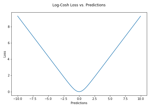

   

   Advantage: $log(cosh(x))$ is approximately equal to $(x\star \star2)/2$ for small $x$ and to $abs(x)-log(2)$ for large $x$. This means that ‘logcosh’ works mostly like the mean squared error, but will not be so strongly affected by the occasional wildly incorrect prediction. It has all the advantages of Huber loss, and it’s twice differentiable everywhere,unlike Huber loss.

   Why do we need a 2nd derivative?
   Many ML model implementations like XGBoost use Newton’s method to find the optimum, which is why the second derivative (Hessian) is needed. For ML frameworks like XGBoost, twice differentiable functions are more favorable.

   But Log-cosh loss isn’t perfect. It still suffers from the problem of gradient and hessian for very large off-target predictions being constant, therefore resulting in the absence of splits for XGBoost.

4. Quantile Loss
   Quantile loss functions turns out to be useful when we are interested in predicting an interval instead of only point predictions. Prediction interval from least square regression is based on an assumption that residuals ($y—\hat{y}$) have constant variance across values of independent variables. We can not trust linear regression models which violate this assumption. We can not also just throw away the idea of fitting linear regression model as baseline by saying that such situations would always be better modeled using non-linear functions or tree based models. This is where quantile loss and quantile regression come to rescue as regression based on quantile loss provides sensible prediction intervals even for residuals with non-constant variance or non-normal distribution.

   Understanding the quantile loss function
   The idea is to choose the quantile value based on whether we want to give more value to positive errors or negative errors. Loss function tries to give different penalties to overestimation and underestimation based on the value of chosen quantile ($\gamma$). For example, a quantile loss function of $\gamma=0.25$ gives more penalty to overestimation and tries to keep prediction values a little below median

   $L_{\gamma}(y,y^p)=\sum_{i=y_i<y^p_i}(\gamma-1)\cdot |y_i-y_i^p|+\sum_{i=y_i\geq y_i^p}(\gamma)\cdot|y_i-y_i^p|$

5. Exponential Loss
   $L(y,f(x))=exp(-yf(x))$