
Introduction
segmentation也是Computer Vision领域一个非常重要的研究方向,和Classification,Detection一起是high-level vision里最重要的方向。我不是主要做Segmentation的,但由于Segmentation的广泛的应用方向(例如自动驾驶的场景感知)和研究热点,本文旨在梳理近些年CV顶会上一些非常有代表性的work。
@LucasXU注:本文长期更新。
Fully Convolutional Networks for Semantic Segmentation
Paper: Fully Convolutional Networks for Semantic Segmentation
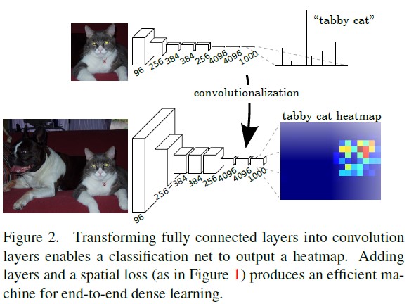
本文针对semantic segmentation问题提出了一个Fully Convolutional Network (FCN),它可以接受任意size的image作为input,然后给出分割后的预测输出。
注:若读者不清楚为啥fully convolutional network能处理arbitrary size input,不妨回想一下经典的detection algorithm SPPNet,因为CNN必须接受fixed size作为input的原因就是后面接了几层fully connected layers,如果整个网络都是全卷积的,那自然就不需要了。
此外,因DCNN提取的hierarchical feature,low-level包含更多细节信息,high-level包含更多semantic meaning。Global information解决了”what”,即input image的semantic meaning,而local information解决了”where”,即包含更多的spatial localization information。而根据DCNN提取feature的层次性特点,因此作者在文中很自然引入了skip architecture,把不同level的feature结合起来以提升segmentation performance。
作者使用的Deep Model依然来自于Classification Model (AlexNet/VGG/GoogLeNet),只是将后面的fully connected layers改成了fully convolutional layers + de-conv来适应segmentation任务。采用反卷积层对最后一个卷积层的feature map进行上采样, 使它恢复到输入图像相同的尺寸,从而可以对每个像素都产生了一个预测, 同时保留了原始输入图像中的空间信息, 最后在上采样的特征图上进行逐像素分类。
Fully convolutional networks
若FCN的loss为最后一层spatial dimension的求和,$l(x;\theta)=\sum_{ij}l^{‘}(x_{ij};\theta)$,那么梯度就可以被计算为每个spatial component的求和。因此将最后一层的receptive fields作为mini-batch的话,在整张图上SGD优化$l$与spatial component上SGD优化$l^{‘}是等效的$。当这些receptive fileds有大量重叠时,layer-by-layer的feedforward computation/BP 比patch-by-patch的计算要高效。
Adapting classifiers for dense prediction
Shift-and-stitch is filter rarefaction
Dense predictions can be obtained from coarse outputs
by stitching together output from shifted versions of the input. If the output is downsampled by a factor of $f$, shift the input $x$ pixels to the right and $y$ pixels down, once for every $(x, y)$ s.t. $0\leq x, y \leq f$. Process each of these $f^2$ inputs, and interlace the outputs so that the predictions correspond to the pixels at the centers of their receptive fields.
Consider a layer (convolution or pooling) with input stride $s$, and a subsequent convolution layer with filter weights $f_{ij}$ (eliding the irrelevant feature dimensions). Setting the lower layer’s input stride to 1 upsamples its output by a factor of $s$. However, convolving the original filter with the upsampled output does not produce the same result as shift-and-stitch, because the original filter only sees a reduced portion of its (now upsampled) input. To reproduce the trick, rarefy the filter by enlarging it as:
$$
f_{ij}^{‘}=\begin{cases}
f_{i/s,j/s} & \text{if $s$ divides both $i$ and $j$}\\
0 & \text{otherwise}
\end{cases}
$$
(with $i$ and $j$ zero-based). Reproducing the full net output of the trick involves repeating this filter enlargement layer-by-layer until all subsampling is removed. (In practice, this can be done efficiently by processing subsampled versions of the upsampled input.)
Upsampling is backwards strided convolution
Another way to connect coarse outputs to dense pixels is interpolation. For instance, simple bilinear interpolation computes each output $y_{ij}$ from the nearest four inputs by a linear map that depends only on the relative positions of the input and output cells.
In a sense, upsampling with factor $f$ is convolution with a fractional input stride of $1/f$. So long as $f$ is integral,a natural way to upsample is therefore backwards convolution (sometimes called deconvolution) with an output stride of $f$. Such an operation is trivial to implement, since it simply reverses the forward and backward passes of convolution. Thus upsampling is performed in-network for end-to-end learning by backpropagation from the pixelwise loss.
Patchwise training is loss sampling
In stochastic optimization, gradient computation is driven by the training distribution. Both patchwise training and fully convolutional training can be made to produce any distribution, although their relative computational efficiency depends on overlap and minibatch size. Whole image fully convolutional training is identical to patchwise training where each batch consists of all the receptive fields of the units below the loss for an image (or collection of images). While this is more efficient than uniform sampling of patches, it reduces the number of possible batches. However, random selection of patches within an image may be recovered simply. Restricting the loss to a randomly sampled subset of its spatial terms (or, equivalently applying a DropConnect mask [36] between the output and the loss) excludes patches from the gradient computation.
Sampling in patchwise training can correct class imbalance [27, 7, 2] and mitigate the spatial correlation of dense patches [28, 15]. In fully convolutional training, class balance can also be achieved by weighting the loss, and loss sampling can be used to address spatial correlation.
Segmentation Architecture
Base network是由AlexNet/VGG/GoogLeNet改动而来,Loss采用per-pixel multinominal logistic loss。整体architecture如下: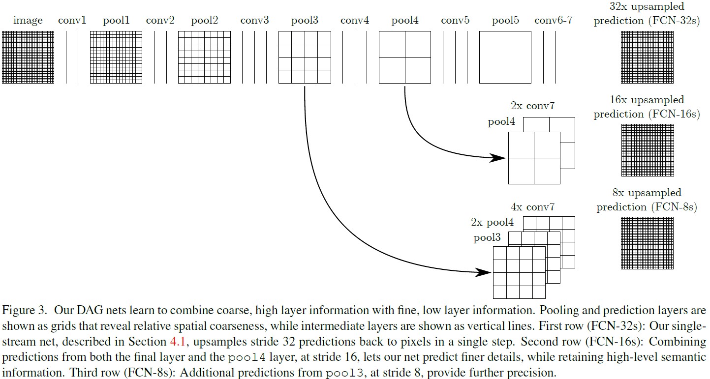
Combining what and where
We address this by adding skips [1] that combine the final prediction layer with lower layers with finer strides. This turns a line topology into a DAG, with edges that skip ahead from lower layers to higher ones (Figure 3). As they see fewer pixels, the finer scale predictions should need fewer layers, so it makes sense to make them from shallower net outputs. Combining fine layers and coarse layers lets the model make local predictions that respect global structure.
We first divide the output stride in half by predicting from a 16 pixel stride layer. We add a $1\times 1$ convolution layer on top of pool-4 to produce additional class predictions. We fuse this output with the predictions computed on top of conv7 (convolutionalized fc7) at stride 32 by adding a $2\times$ upsampling layer and summing both predictions (see Figure 3). We initialize the $2\times$ upsampling to bilinear interpolation, but allow the parameters to be learned as described in Section 3.3. Finally, the stride 16 predictions are upsampled back to the image. We call this net FCN-16s. FCN-16s is learned end-to-end, initialized with the parameters of the last,coarser net, which we now call FCN-32s. The new parameters acting on pool4 are zeroinitialized so that the net starts with unmodified predictions. The learning rate is decreased by a factor of 100.
Mask RCNN
Paper: Mask r-cnn
Mask RCNN是Kaiming He发表在ICCV 2017上的Paper,在Segmentation和Detection任务上均取得了state-of-the-art的成绩。本文就来对Mask RCNN进行一下细致的讲解。
What is Mask RCNN?
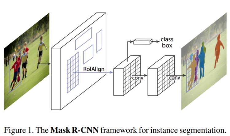
Mask RCNN可以看作是Faster RCNN + Mask branch for Segmentation。Mask branch是应用在每一个RoI上的small FCN,用来预测segmentation mask。Faster RCNN是一种非常优秀的object detection framework,但是却并不适合pixel-to-pixel alignment,原因就在于Faster RCNN中的RoI Pooling Layer perform coarse spatial quantization for feature extraction。为了修复misalignment问题,作者在Mask RCNN中引入了RoIAlign来保留exact spatial locations。此外,作者还发现RoIAlign对mask和classification prediction的解耦非常重要。
We predict a binary mask for each class independently, without competition among classes, and rely on the network’s RoI classification branch to predict the category. In contrast, FCNs usually perform per-pixel multi-class categorization, which couples segmentation and classification, and based on our experiments works poorly for instance segmentation.
Delve into Mask RCNN
熟悉Faster RCNN的同学都应该知道,Faster RCNN=RPN + Fast RCNN,即RPN通过sliding window的方式在feature map上生成region proposal,然后同时做bbox offset regression + classification。之前的segmentation算法会将object classification和segmentation同时处理(类似于Fast RCNN中的bbox regression和object classification做Multi-task training那样同时处理)。Mask RCNN也采取了two-stage的方法:即在第一个stage运行RPN,第二个stage做bbox offset regression + object classification。同时Mask Branch也针对每一个RoI输出binary mask。
所以,整体的Loss Function定义为:
$$
L=L_{cls} + L_{box} + L_{mask}
$$
其中,$L_{cls}$和$L_{box}$分别是Softmax Loss和Smooth L1 Loss。对于每个RoI,Mask branch产生$Km^2$-dimensional outputs,也就是说对$m\times m$ resolution encode $K$个 binary mask,分别对应$K$个classes。$L_{mask}$处理方式如下:
We apply a per-pixel sigmoid, and define $L_{mask}$ as the average binary cross-entropy loss. For an RoI associated with ground-truth class k, Lmask is only defined on the k-th mask (other mask outputs do not contribute to the loss).
Our definition of $L_{mask}$ allows the network to generate masks for every class without competition among classes. We rely on the dedicated classification branch to predict the class label used to select the output mask. This decouples mask and class prediction. This is different from common practice when applying FCNs [24] to semantic segmentation, which typically uses a per-pixel softmax and a multinomial cross-entropy loss. In that case, masks across classes compete; in our case, with a per-pixel sigmoid and a binary loss, they do not. We show by experiments that this formulation is key for good instance segmentation results.
Mask Representation
A mask encodes an input object’s spatial layout. Thus, unlike class labels or box offsets that are inevitably collapsed into short output vectors by fully-connected (fc) layers, extracting the spatial structure of masks can be addressed naturally by the pixel-to-pixel correspondence provided by convolutions.
Specifically, we predict an $m\times m$ mask from each RoI using an FCN [24]. This allows each layer in the mask branch to maintain the explicit $m\times m$ object spatial layout without collapsing it into a vector representation that lacks spatial dimensions. Unlike previous methods that resort to fc layers for mask prediction [27, 28, 7], our fully convolutional representation requires fewer parameters, and is more accurate as demonstrated by experiments.
This pixel-to-pixel behavior requires our RoI features, which themselves are small feature maps, to be well aligned to faithfully preserve the explicit per-pixel spatial correspondence. This motivated us to develop the following RoIAlign layer that plays a key role in mask prediction.
RoIAlign
RoIPool [9] is a standard operation for extracting a small feature map (e.g., $7\times 7$) from each RoI. RoIPool first quantizes a floating-number RoI to the discrete granularity of the feature map, this quantized RoI is then subdivided into spatial bins which are themselves quantized, and finally feature values covered by each bin are aggregated (usually by max pooling). Quantization is performed, e.g., on a continuous coordinate x by computing $[x/16]$, where 16 is a feature map stride and $[\cdot]$ is rounding; likewise, quantization is performed when dividing into bins (e.g., $7\times 7$). These quantizations introduce misalignments between the RoI and the extracted features. While this may not impact classification, which is robust to small translations, it has a large negative effect on predicting pixel-accurate masks.
To address this, we propose an RoIAlign layer that removes the harsh quantization of RoIPool, properly aligning the extracted features with the input. Our proposed change is simple: we avoid any quantization of the RoI boundaries or bins (i.e., we use $x/16$ instead of $[x/16]$). We use bilinear interpolation [18] to compute the exact values of the input features at four regularly sampled locations in each RoI bin, and aggregate the result (using max or average).
Ablation Study
Multinomial vs. Independent Masks
Mask R-CNN decouples mask and class prediction: as the existing box branch predicts the class label, we generate a mask for each class without competition among classes (by a per-pixel sigmoid and a binary loss). In Table 2b, we compare this to using a per-pixel softmax and a multinomial loss (as commonly used in FCN [24]). This alternative couples the tasks of mask and class prediction, and results in a severe loss in mask AP (5.5 points). This suggests that once the instance has been classified as a whole (by the box branch), it is sufficient to predict a binary mask without concern for the categories, which makes the model easier to train.
Class-Specific vs. Class-Agnostic Masks
Our default instantiation predicts class-specific masks, i.e., one $m\times m$ mask per class. Interestingly, Mask R-CNN with classagnostic masks (i.e., predicting a single m×m output regardless of class) is nearly as effective: it has 29.7 mask AP vs. 30.3 for the class-specific counterpart on ResNet-50-C4. This further highlights the division of labor in our approach which largely decouples classification and segmentation.
Mask Branch
Segmentation is a pixel-to-pixel task and we exploit the spatial layout of masks by using an FCN. In Table 2e, we compare multi-layer perceptrons (MLP) and FCNs, using a ResNet-50-FPN backbone. Using FCNs gives a 2.1 mask AP gain over MLPs. We note that we choose this backbone so that the conv layers of the FCN head are not pre-trained, for a fair comparison with MLP.
FC_DenseNet
Paper: The one hundred layers tiramisu: Fully convolutional densenets for semantic segmentation
Code: Github
本篇介绍一下CVPR Workshop 2017 上面的一篇paper,idea非常简单,就是单纯地将DenseNet扩展为FCN架构,然后取得了很不错的效果。笔者认为,该算法能work很大程度上取决于优秀的backbone——DenseNet,以及在segmentation非常work的工作——FCN。本文novelty很一般,但鉴于工程中实际上并不需要太复杂的方法,所以还是讲解一下吧。
先回顾一下FCN-based segmentation methods:
(1) downsampling layers用来提取coarse semantic features
(2) upsampling layers恢复到和input image相同size的output;因low-level features包含很多细节信息,所以常常会再网络中加入skip connection结构
(3) CRF(Conditional Random Field)用于提纯上一步较coarse的prediction
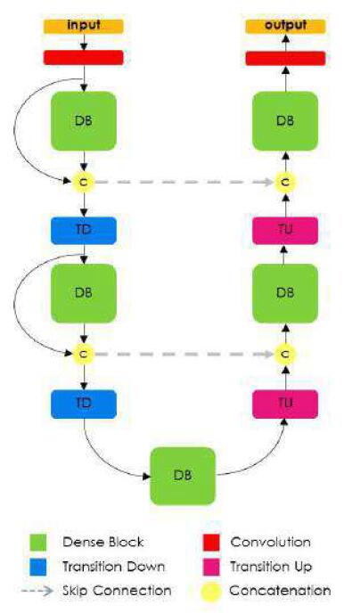
本文,作者对DenseNet进行了改进:首先将其改为FCN结构,但只在相邻dense block采用upsampling operation,对于相同dimension的feature map利用skip connection连接起来,来获取multi-scale的information。整体网络也借鉴了UNet的结构:
Reference
- Long J, Shelhamer E, Darrell T. Fully convolutional networks for semantic segmentation[C]//Proceedings of the IEEE conference on computer vision and pattern recognition. 2015: 3431-3440.
- He, Kaiming, et al. “Mask r-cnn.” Computer Vision (ICCV), 2017 IEEE International Conference on. IEEE, 2017.
- Jégou S, Drozdzal M, Vazquez D, et al. The one hundred layers tiramisu: Fully convolutional densenets for semantic segmentation[C]//Proceedings of the IEEE Conference on Computer Vision and Pattern Recognition Workshops. 2017: 11-19.
- Ronneberger O, Fischer P, Brox T. U-net: Convolutional networks for biomedical image segmentation[C]//International Conference on Medical image computing and computer-assisted intervention. Springer, Cham, 2015: 234-241.