[DL] Architecture

Introduction

Deep Learning有三宝：Network Architecture，Loss Function and Optimization。对于大多数人而言，Optimization门槛还是很高的（需要非常深厚的数学功底），所以绝大多数的Paper偏向还是设计更好的Network Architecture或者堆更加精巧的Loss Function。Ian Goodfellow大佬也曾说过：现如今Deep Learning的繁荣，网络结构探究的贡献度远远高于优化算法的贡献度。所以本文旨在梳理从AlexNet到CliqueNet这些经典的work。

@LucasX注：对于优化算法，可参考我的这一篇文章。

AlexNet

Paper: Imagenet classification with deep convolutional neural networks

AlexNet可以看作是Deep Learning在Large Scale Image Classification Task上第一次大放异彩。也是从AlexNet起，越来越多的Computer Vision Researcher开始将重心由设计更好的hand-crafted features转为设计更加精巧的网络结构。因此AlexNet是具备划时代意义的经典work。

AlexNet整体结构其实非常非常简单，5层conv + 3层FC + Softmax。AlexNet使用了ReLU来代替Sigmoid作为non-linearity transformation，并且使用双GPU训练，以及一系列的Data Augmentation操作，Dropout，对于今天的工作仍然具备很深远的影响。

VGG

Paper: Very deep convolutional networks for large-scale image recognition

VGG也是一篇非常经典的工作，并且在今天的很多任务上依旧可以看到VGG的影子。不同于AlexNet，VGG使用了非常小的Filter($3\times 3$)，以及类似于basic block结构(读者不妨回想一下GoogLeNet、ResNet、ResNeXt、DenseNet是不是也是由一系列block堆积而成的)。

不妨思考一下为啥要用$3\times 3$的卷积核呢？

1. 两个堆叠的$3\times 3$卷积核对应$5\times 5$的receptive field。而三个$3\times 3$卷积核对应$7\times 7$的receptive field。那为啥不直接用$7\times 7$卷积呢？原因就在于通过堆叠的3个$3\times 3$卷积核，我们引入了更多的non-linearity transformation，这有助于我们的网络学习更加discriminative的特征表达。
2. 减少了参数：3个channel为$C$的$3\times 3$卷积的参数为: $3(3^2C^2)=27C^2$。而一个channel为$C$的$7\times 7$卷积的参数为: $7^2C^2=49C^2$。

   This can be seen as imposing a regularisation on the $7\times 7$ conv. filters, forcing them to have a decomposition through the $3\times 3$ filters (with non-linearity injected in between)

Network in network

Paper: Network in network

Network in network (NIN) 也是深度学习网络结构设计领域一篇非常insightful的paper，并且直接启发了GoogLeNet、CAM等算法的设计，NIN主要的contribution如下：

1. 一种新型引入non-linearity transformation的方法：每个conv layer后接一个小型的MLP(即本文title Network in network)，以sliding window的方式在conv layer的输出进行滑动；相比之下，传统conv可视为一种generalized linear model，而没有mlpconv这么多非线性变换能力。
2. 著名的$1\times 1$ conv，GoogLeNet、ShuffleNet中大量使用$1\times 1$ conv来进行升维、降维；$1\times 1$ conv也能起到整合cross channel information的作用。
3. Global Average Pooling，GAP可视为一种Regularization方法。

NIN的网络结构如下：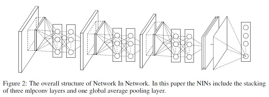

Global Average Pooling

GAP的优点：

1. GAP is more native to the convolution structure by enforcing correspondences between feature maps and categories. Thus the feature maps can be easily interpreted as categories confidence maps.
2. No parameters needed to optimize in GAP thus avoid overfitting.
3. GAP sums out spatial information, thus it is more robust to spatial translations of the input.

We can see global average pooling as a structural regularizer that explicitly enforces feature maps to be confidence maps of concepts (categories). This is made possible by the mlpconv layers as they makes better approximation to the confidence maps than GLMs.

Global Average Pooling as a Regularizer

GAP和FC作用相似，都是对features进行一个linear combination，但是差异存在于transformation matrix。GAP中transformation matrix是固定的；而FC中是通过BP学习的。

最后，通过可视化实验分析，作者发现，classification experiment中，activiation激活最高的区域恰恰是原图中object存在的区域，那说明GAP encode了非常强的category information，那可不可以用来做weakly supervised detection呢？答案是当然可以，于是CAM就是受了本文的启发做出来的。

GoogLeNet

Paper: Going deeper with convolutions

因DCNN在一系列CV任务上均取得了非常好的效果，所以大家开始将精力由hand-crafted features转换到network architecture上来了。GoogLeNet也是经典网络中一个非常值得关注的模型，其中值得关注的设计就是Multi-branch + Feature Concatenation，这是今天很多深度学习算法也依旧在使用的方法。GoogLeNet中，作者大量使用了$1\times 1$ conv (注：$1\times 1$ conv最先来自Network in network)，这样有以下好处：

• 作为dimension reduction来remove computational bottlenecks
• 既然computational bottlenecks减少了，那么在相同FLOPs下，我们可以设计更加deep的网络结构，从而辅助更好的representation learning

Inception Module的基础结构如下图所示：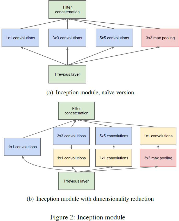

在走每一个$3\times 3$和$5\times 5$ conv之前，先过一遍$1\times 1$ conv，一方面可以起到dimension reduction的作用；另一方面也引入了更多的non-linearity transformation，而这对于整个网络的representation learning ability是非常重要的(这个套路基本和Network in network一样，感兴趣的读者可以去阅读Network in network原文)。

GoogLeNet就是通过一系列的Inception Module堆叠而成(读者不妨再仔细思考一下，VGG/ResNet/ResNeXt等等网络是不是也是由一系列小block堆叠而成？)。此外，因GoogLeNet是Multi-branch的结构，所以作者在中间层也添加了classification layer作为supervision来辅助gradient flow(读者不妨回忆一下，经典的人脸识别算法DeepID是不是也是这么做的？)。

ResNet

Paper: Deep Residual Learning for Image Recognition

笔者认为，ResNet可以称得上是自AlexNet以来，Deep Learning发展最insightful的idea，ResNet的主角shortcut至今也被广泛应用于Deep Architecture的设计中(如DenseNet, CliqueNet, Deep Layer Aggregation等)。
此前的网络设计趋势是“越来越深”，但神经网络的设计真的就如同段子所言“一层一层往上堆叠就好了吗？”显然不是的，ResNet作者Kaiming He大神在Paper中做了一些实验，验证了当Network越来越深时，Accuracy就饱和了，然后迅速下降，值得一提的是这种性能下降并不是由于参数过多随之而来的overfitting造成的。

What is Residual Network?

设想DNN的目的是为了学习某种function $\mathcal{H}(x)$，作者并没有直接设计DNN Architecture去学习这种function，而是先学习另一种function $\mathcal{F}(x):=\mathcal{H}(x) - x$，那么原来的$\mathcal{H}(x)$是不是就可以表示成$\mathcal{F}(x)+x$。作者假设这种结构比原先的$\mathcal{H}(x)$更容易优化。

例如，若某种identity mapping是最优的，那么，将残差push到0要比通过一系列non-linearity transformation来学习identity mapping更为高效。

Shortcut可以表示成如下结构：
$$
y=\mathcal{F}(x, \{W_i\}) + x
$$
$\mathcal{F}(x, \{W_i\})$可以表示多个conv layers，两个feature map通过channel by channel element-wise 叠加。

网络结构的设计方面，依旧是参考了著名的VGG，即：使用大量$3\times 3$ filters并且遵循这两条原则：

1. 对于输出相同feature map size的层使用相同数量的filter
2. 若feature map size减半，则filter的数量则翻倍，来维持每一层的time complexity

对于feature map dimension相同的情况，则只需要element-wise addition即可；若feature map dimension double了，可以采取zero padding来增加dimension，或者采用$1\times 1$ conv来进行升维。

ResNet到这里基本就介绍完了，实验部分当然是在classification/detection/segmentation task上吊打了当前所有的state-of-the-art。ResNet很简单的idea对不对？不得不佩服一下Kaiming，他的东西总是简单而有效！

ShuffleNet

在Computer Vision领域，除了像AlexNet、VGG、GoogLeNet、ResNet、DenseNet、CliqueNet等一系列比较“重量级”的网络结构之外，也有一些非常轻量级的模型，而轻量级模型对于移动设备而言无疑是非常重要的。这里就介绍一下轻量级模型的代表作之一：ShuffleNet。

Paper: ShuffleNet: An Extremely Efficient Convolutional Neural Network for Mobile Devices

What is ShuffleNet?

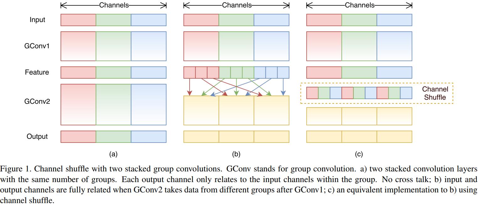
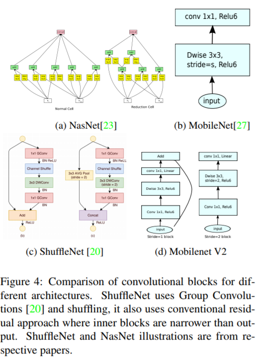
ShuffleNet结构最重要的两个部分就是Pointwise Group Convolution和Channel Shuffle。

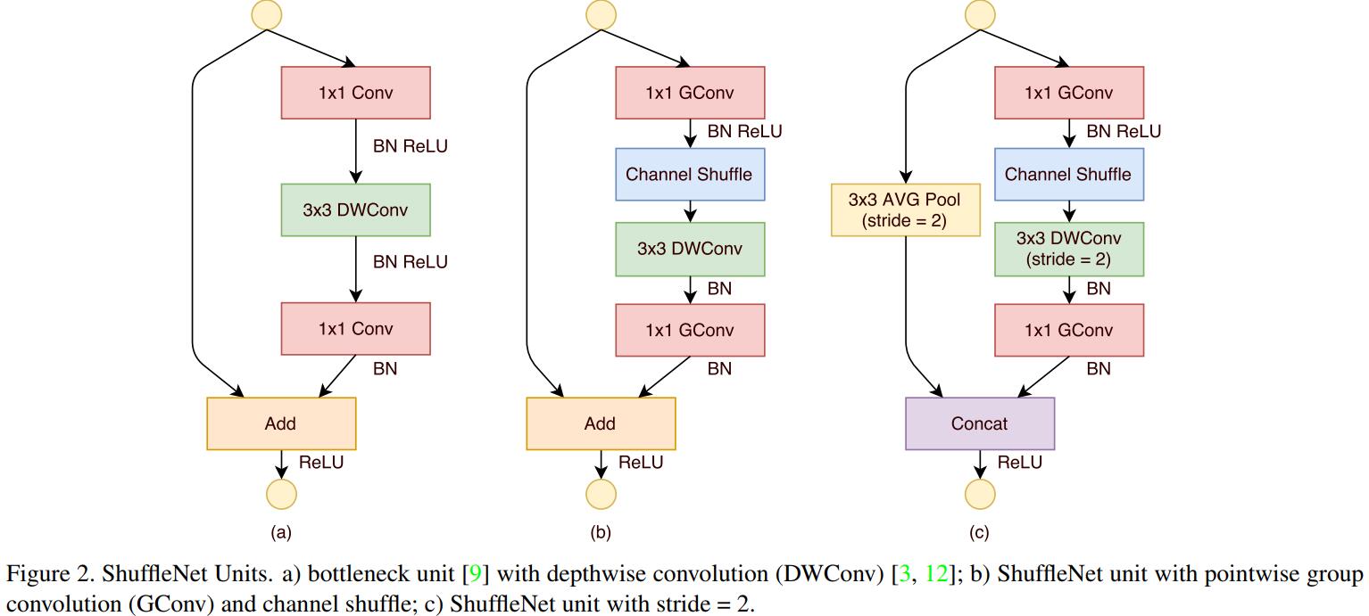
Given a computational budget, ShuffleNet can use wider feature maps. We find this is critical for small networks, as tiny networks usually have an insufficient number of channels to process the information. In addition, in ShuffleNet depthwise convolution only performs on bottleneck feature maps. Even though depthwise convolution usually has very low theoretical complexity, we find it difficult to efficiently implement on lowpower mobile devices, which may result from a worse computation/memory access ratio compared with other dense operations.

Advantages of Point-Wise Convolution

Note that group convolution allows more feature map channels for a given complexity constraint, so we hypothesize that the performance gain comes from wider feature maps which help to encode more information. In addition, a smaller network involves thinner feature maps, meaning it benefits more from enlarged feature maps.

Channel Shuffle vs. No Shuffle

The purpose of shuffle operation is to enable cross-group information flow for multiple group convolution layers. The evaluations are performed under three different scales of complexity. It is clear that channel shuffle consistently boosts classification scores for different settings. Especially, when group number is relatively large (e.g. g = 8), models with channel shuffle outperform the counterparts by a significant margin, which shows the importance of cross-group information interchange.

MobileNet V1

Paper: MobileNets: Efficient Convolutional Neural Networks for Mobile Vision Applications

CNN驱动了许多视觉任务的飞速发展，然而传统结构例如ResNet、Inception、VGG等FLOP非常大，这使得对于移动端和嵌入式设备的训练与部署变得非常困难。所以近些年来，轻量级网络的设计也成为了一个非常热门的研究方向，MobileNet和ShuffleNet就是其中的代表。前面我们已经介绍了ShuffleNet，本篇我们就大致回顾一下MobileNet。

Depth-wise Separable Convolution

MobileNet最主要的结构就是Depth-wise Separable Convolution。DW Conv为什么能减少model size呢？我们不妨先来细致分析一下传统的卷积需要多少参数:
假设传统卷积层接受一个$D_F\times D_F\times M$的feature map $F$作为输入，然后输出$D_G\times D_G\times N$的feature map $G$，所以卷积核的size是$D_K\times D_K\times M\times N$，所以需要的计算量为：$D_K\times D_K\times M\times N\times D_F\times D_F$，所以Computational Cost依赖于input channel $M$，output channel $N$，卷积核尺寸$D_K\times D_K$和feature map的尺寸$D_F\times D_F$。

但是MobileNet应用Depth-wise Conv来对Kernel Size和Output Channel进行了解耦。传统Conv Operation通过filters来对features进行filter，然后重组(Combinations)以形成新的representations。Filtering和Combinations可通过DW Separable Conv来分成两步进行。

Depth-wise Separable Convolution由两层组成：Depth-wise Conv + Point-wise Conv。DW Conv对于每个channel应用单个filter，PW Conv (a simple $1\times 1$ Conv)用来建立DW layer输出的linear combination。DW Conv的Computational Cost为: $D_K\times D_K\times M\times D_F\times D_F$，与传统Conv相比低了$N$倍。

DW Conv虽然高效，然而它仅仅filter了input channel，却没有对其进行combination，所以需要额外的layer来对DW Conv后的feature进行linear combination来产生新的representation，这就是基于$1\times 1$ Conv的PW Conv。

The combination of depthwise convolution and $1\times 1$ (pointwise) convolution is called depthwise separable convolution.

DW Separable Conv的Computational Cost为：
$D_K\times D_K \times M\times D_F \times D_F + M\times N\times D_F\times D_F$，前者为DW Conv的cost，后者为PW Conv的cost。

By expressing convolution as a two step process of filtering and combining we get a reduction in computation of:
$$
\frac{D_K\times D_K \times M\times D_F \times D_F + M\times N\times D_F\times D_F}{D_K\times D_K \times M\times N\times D_F \times D_F}=\frac{1}{N} + \frac{1}{D_K^2}
$$
可以看到，Depth-wise Separable Conv的计算量仅仅为传统Conv的$\frac{1}{N} + \frac{1}{D_K^2}$。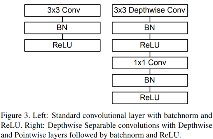

Width Multiplier: Thinner Models

In order to construct these smaller and less computationally expensive models we introduce a very simple parameter $\alpha$ called width multiplier. The role of the width multiplier α is to thin a network uniformly at each layer. The computational cost of a depthwise separable convolution with width multiplier $\alpha$ is:

$D_K\times D_K\times \alpha M\times D_F\times D_F +\alpha M\times \alpha N + D_F\times D_F$

where $\alpha\in (0, 1]$ with typical settings of 1, 0.75, 0.5 and 0.25. $\alpha = 1$ is the baseline MobileNet and $\alpha < 1$ are reduced MobileNets. Width multiplier has the effect of reducing computational cost and the number of parameters quadratically by roughly $\alpha^2$ . Width multiplier can be applied to any model structure to define a new smaller model with a reasonable accuracy, latency and size trade off. It is used to define a new reduced structure that needs to be trained from scratch.

Resolution Multiplier: Reduced Representation

The second hyper-parameter to reduce the computational cost of a neural network is a resolution multiplier $\rho$. We apply this to the input image and the internal representation of every layer is subsequently reduced by the same multiplier. In practice we implicitly set $\rho$ by setting the input resolution. We can now express the computational cost for the core layers of our network as depthwise separable convolutions with width multiplier $\alpha$ and resolution multiplier $\rho$:

$D_K\times D_K\times \alpha M\times \rho D_F\times \rho D_F +\alpha M\times \alpha N + \rho D_F\times \rho D_F$

where $\rho\in (0, 1]$ which is typically set implicitly so that the input resolution of the network is 224, 192, 160 or 128. $\rho = 1$ is the baseline MobileNet and ρ < 1 are reduced computation MobileNets. Resolution multiplier has the effect of reducing computational cost by $\rho^2$.

MobileNet V2

Paper: MobileNetV2: Inverted Residuals and Linear Bottlenecks

MobileNet V2是发表在CVPR2018上的Paper，在移动端网络的设计方面又向前走了一步。MobileNet V2最大的contribution如下:

Our main contribution is a novel layer module: the inverted residual with linear bottleneck. This module takes as an input a low-dimensional compressed representation which is first expanded to high dimension and filtered with a lightweight depthwise convolution. Features are subsequently projected back to a low-dimensional representation with a linear convolution.

Preliminaries, discussion and intuition

Depthwise Separable Convolutions

说起Light-weighted Architecture呢，DW Conv是必不可少的组件了，同理，MobileNet V2也是基于DW Conv做的改进。

The basic idea is to replace a full convolutional operator with a factorized version that splits convolution into two separate layers. The first layer is called a depthwise convolution, it performs lightweight filtering by applying a single convolutional filter per input channel. The second layer is a $1\times 1$ convolution, called a pointwise convolution, which is responsible for building new features through computing linear combinations of the input channels.

传统Conv接受一个$h_i\times w_i\times d_i$输入，应用卷积核$K\in \mathcal{R}^{k\times k\times d_i\times d_j}$来产生$h_i\times w_i\times d_j$的输出。所以传统Conv的Computational Cost为：$h_i\times w_i\times d_i \times d_j\times k\times k$。而DW Separable Conv的Computational Cost仅仅为：$h_i\times w_i\times d_i(k^2+d_j)$，减少了将近$k^2$倍的计算量。

Linear Bottlenecks

It has been long assumed that manifolds of interest in neural networks could be embedded in low-dimensional subspaces. In other words, when we look at all individual d-channel pixels of a deep convolutional layer, the information encoded in those values actually lie in some manifold, which in turn is embeddable into a low-dimensional subspace.

DCNN的架构大致是这样的：Conv + ReLU + (Pool) + (FC) + Softmax。DNN之所以拟合能力超强，原因就在于non-linearity transformation，而由于gradient vanishing/exploding的原因，Sigmoid已经淡出了历史舞台，取而代之的是ReLU。我们来分析分析ReLU有什么缺点：

It is easy to see that in general if a result of a layer transformation ReLU(Bx) has a non-zero volume S, the points mapped to interior S are obtained via a linear transformation B of the input, thus indicating that the part of the input space corresponding to the full dimensional output, is limited to a linear transformation. In other words, deep networks only have the power of a linear classifier on the non-zero volume part of the output domain.

On the other hand, when ReLU collapses the channel, it inevitably loses information in that channel. However if we have lots of channels, and there is a a structure in the activation manifold that information might still be preserved in the other channels. In supplemental materials, we show that if the input manifold can be embedded into a significantly lower-dimensional subspace of the activation space then the ReLU transformation preserves the information while introducing the needed complexity into the set of expressible functions.

简而言之，ReLU有以下两种性质：

1. 若Manifold of Interest在ReLU之后非零，那么它就相当于是一个线性变换。
2. ReLU能够保存input manifold完整的信息，但是当且仅当input manifold位于input space的低维子空间中时。

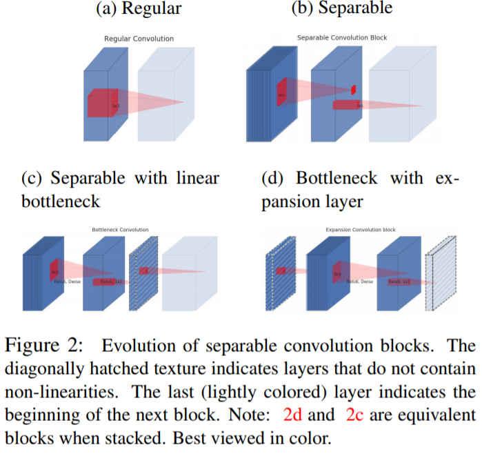
Inverted residuals

The bottleneck blocks appear similar to residual block where each block contains an input followed by several bottlenecks then followed by expansion [8]. However, inspired by the intuition that the bottlenecks actually contain all the necessary information, while an expansion layer acts merely as an implementation detail that accompanies a non-linear transformation of the tensor, we use shortcuts directly between the bottlenecks.

回想一下，MobileNet V1的结构就是一个普通的feedforwad network，而shortcut在ResNet里已经被证明是非常effective的了，所以MobileNet V2自然而然地引入了skip connection了。并且，因为ResNet采用的是vanilla conv，为了降低整个网络的计算量，所以设计成了bottleneck的结构（即两头宽中间窄）；而在MobileNet V2中，因为采用的是depth-wise separable conv，使得计算量大大降低，故采用了inverted residual的结构（即两头窄中间宽）。

MobileNet V2 Architecture

We use ReLU6 as the non-linearity because of its robustness when used with low-precision computation [27]. We always use kernel size $3\times 3$ as is standard for modern networks, and utilize dropout and batch normalization during training.

ResNeXt

Paper: Aggregated Residual Transformations for Deep Neural Networks

Introduction

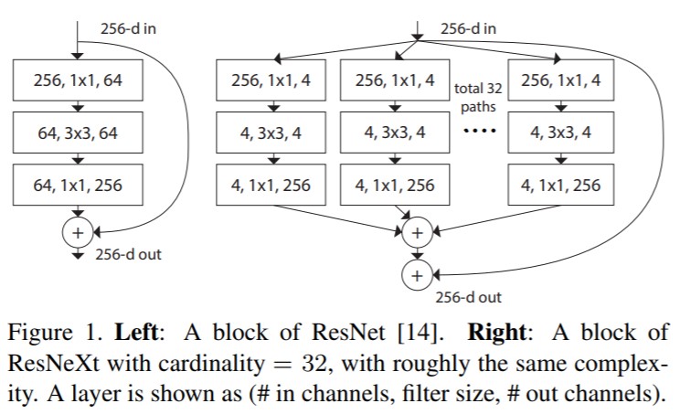
自AlexNet以来，Deep Learning涌现了一大批设计优良的网络(如VGG，Inception，ResNet等)。ResNeXt则在ResNet的基础上，一定程度上参考了Inception的设计，即split-transform-merge。

The Core of ResNeXt

Unlike VGG-nets, the family of Inception models [38, 17, 39, 37] have demonstrated that carefully designed topologies are able to achieve compelling accuracy with low theoretical complexity. The Inception models have evolved over time [38, 39], but an important common property is a split-transform-merge strategy. In an Inception module, the input is split into a few lower-dimensional embeddings (by 1×1 convolutions), transformed by a set of specialized filters (3×3, 5×5, etc.), and merged by concatenation. It can be shown that the solution space of this architecture is a strict subspace of the solution space of a single large layer (e.g., 5×5) operating on a high-dimensional embedding. The split-transform-merge behavior of Inception modules is expected to approach the representational power of large and dense layers, but at a considerably lower computational complexity.

尽管Inception的split-transform-merge策略是非常行之有效的，但是该网络结构过于复杂，人工设计的痕迹过重(相比之下VGG和ResNet则是由相同的block stacking而成)，给人的感觉就是专门为了ImageNet去做的优化，所以当你想要迁移到其他的dataset时就会比较麻烦。因此，ResNeXt的设计就是：在VGG/ResNet的stacking block的基础上，融合进了Inception的split-transform-merge策略。这就是ResNeXt的基础idea。作者在实验中发现cardinality (the size of the set of transformations)对performance的影响是最大的，甚至要大于width和depth。

Our method harnesses additions to aggregate a set of transformations. But we argue that it is imprecise to view our method as ensembling, because the members to be aggregated are trained jointly, not independently.

The above operation can be recast as a combination of splitting, transforming, and aggregating.

1. Splitting: the vector $x$ is sliced as a low-dimensional embedding, and in the above, it is a single-dimension subspace $x_i$.
2. Transforming: the low-dimensional representation is transformed, and in the above, it is simply scaled: $w_i x_i$.
3. Aggregating: the transformations in all embeddings are aggregated by $\sum_{i=1}^D$.

若将$W$更换为更一般的形式，即任意一种function mapping: $\mathcal{T}(x)$，那么aggregated transformations就变成了:
$$
\mathcal{F}(x)=\sum_{i=1}^C \mathcal{T}_i(x)
$$
其中$\mathcal{T}_i$可以将$x$映射到低维空间。$C$是transformation的size，也就是本文主角——cardinality。

In Eqn.(2), $C$ is the size of the set of transformations to be aggregated. We refer to $C$ as cardinality [2]. In Eqn.(2) $C$ is in a position similar to $D$ in Eqn.(1), but $C$ need not equal $D$ and can be an arbitrary number. While the dimension of width is related to the number of simple transformations (inner product), we argue that the dimension of cardinality controls the number of more complex transformations. We show by experiments that cardinality is an essential dimension and can be more effective than the dimensions of width and depth.

那么在ResNet的identical mapping背景下，就变成了这样一种熟悉的结构：
$$
y=x+\sum_{i=1}^C \mathcal{T}_i(x)
$$

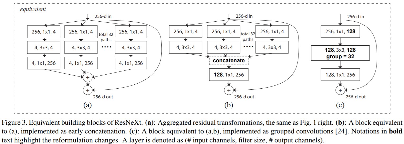
Relation to Grouped Convolutions. The above module becomes more succinct using the notation of grouped convolutions [24]. This reformulation is illustrated in Fig. 3(c). All the low-dimensional embeddings (the first $1\times 1$ layers) can be replaced by a single, wider layer (e.g., $1\times 1$, 128-d in Fig 3(c)). Splitting is essentially done by the grouped convolutional layer when it divides its input channels into groups. The grouped convolutional layer in Fig. 3(c) performs 32 groups of convolutions whose input and output channels are 4-dimensional. The grouped convolutional layer concatenates them as the outputs of the layer. The block in Fig. 3(c) looks like the original bottleneck residual block in Fig. 1(left), except that Fig. 3(c) is a wider but sparsely connected module.

Xception

Paper: Xception: Deep Learning with Depthwise Separable Convolutions

Xception，即Extreme Inception，听名字也知道是Google家的模型啦。我们前面已经提到过，GoogLeNet(即Inception v1)，是由一系列Inception Block堆积而成的，所以Xception自然也是由一系列basic block堆积而成的。只不过，作者将depth-wise separable convolution视为一个Inception module。既然用到了depth-wise separable convolution，读者自然也就容易联想到Xception也属于一种light-weighted architecture了。此外，我们都知道，一个deep model的learning ability是与其capacity有很大关联性的，而Xception与它的前辈Inception v3在参数量上几乎是一样的，也就是说model capacity几乎一致。然而Xception却能带来显著的提升，这就说明Xception相比于Inception v3做到了更加高效的参数利用。

Basic

回想一下，对于一个常规的conv layer，它试图在3D空间中学习filters，其中2D为width and height，另外1D为channel。因此一个conv kernel需要同时处理cross-channel correlation和spatial correlation。Inception module的想法是通过将其显式地分解为一系列独立处理cross-channel correlation和spatial correlation的操作，来使这个过程更容易、更有效。也就是说，Inception在设计之初就是向着cross-channel correlation和spatial correlation互相解耦这个方向的，所以不将cross-channel correlation和spatial correlation协同优化或许是更好的选择。Xception module和depth-wise separable convolution主要有以下两点区别：

• operation的顺序：depth-wise convolution通常先进行channel-wise spatial convolution，再进行$1\times 1$ conv；而Xception module先进行$1\times 1$ conv。
• 在Inception module中，每个operation后面都跟了ReLU，而depth-wise separable convolution后面没有接non-linearity transformation，因此Inception module的非线性能力会更强一些。

其中，第一点是无关紧要的(因为既然是一系列block堆叠而成，那么我假设将第$n$个block的后半部分和第$n+1$个block的前半部分视为一个block呢？顺序是不是就不care了！)；但是第二点引入更多的non-linearity transformation是非常重要的。

The Xception Architecture

作者主要基于这样一种假设：CNN中feature map的cross-channel correlation和spatial correlation能够完全地被解耦，此外，既然Kaiming大神验证了skip connection在DNN中的有效性，因此Xception自然也加入了shortcut结构。网络结构图和data flow如下图所示：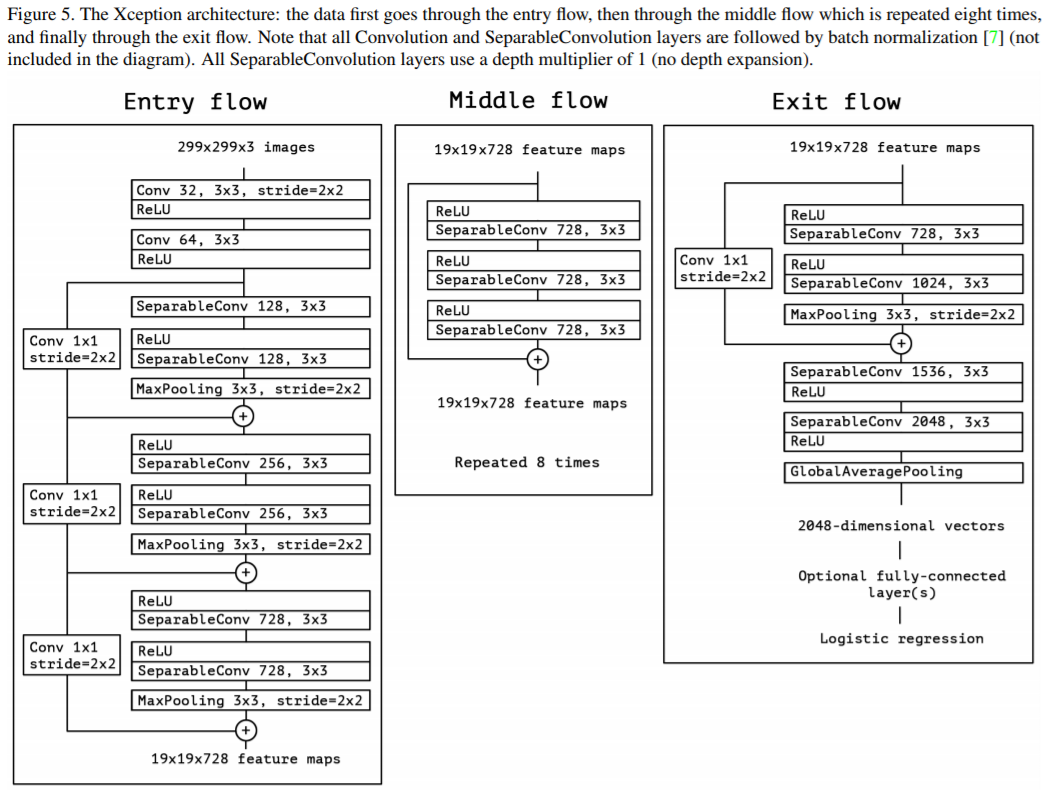

实验结果当然是各种好了，值得一提的是：当时GoogLeNet是在中间层也添加了classification layer来辅助信息BP，这种additional classification layer可视为一种Regularization，但是作者在实验中并没有添加这种额外的auxiliary loss tower(读者不妨猜想一下原因？可能是因为当时还没有出现residual connection这种简单而有效的结构，所以在网络很deep的时候，需要在中间层施加loss layer来辅助梯度流通，但是自打residual shortcut被引进后，自然而然也就不需要了)。

Effect of an intermediate activation after pointwise convolutions

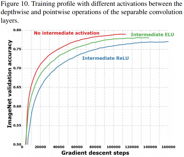
从上图可以看到，没有intermediate activation会带来更快的收敛和更好的performance。作者也分析了这个原因：

It may be that the depth of the intermediate feature spaces on which spatial convolutions are applied is critical to the usefulness of the non-linearity: for deep feature spaces (e.g. those found in Inception modules) the non-linearity is helpful, but for shallow ones (e.g. the 1-channel deep feature spaces of depthwise separable convolutions) it becomes harmful, possibly due to a loss of information.

简而言之，可能在deeper architecture会有用，但是在shallower architecture中引入过多的non-linearity transformation会带来information loss。

DenseNet

Paper: Densely Connected Convolutional Networks

What is DenseNet?

DenseNet是CVPR2017 Best Paper，是继ResNet之后更加优秀的网络。前面我们已经介绍过，ResNet一定程度上解决了gradient vanishing的问题，通过ResNet中的identical mapping使得网络深度可以到达上千层。那么DenseNet又做了哪些改进呢？本文为你一一解答！

在介绍DenseNet之前，我们先回顾一下ResNet做了什么改动，当shortcuts还未被引入DCNN之前，AlexNet/VGG/GoogLeNet都属于构造比较简单的feedforward network，即信息一层一层往前传播，在BP时梯度一层一层往后传，但是这样在网络结构很深的时候，就会存在gradient vanishing的问题。所以Kaiming He创造性地引入了skip connection，来使得信息可以从第$i$层之间做identical mapping传播到第$i+t$层，这样就保证了信息的高效流通。

而DenseNet，就是把这种skip connection做到了极致。为了保证信息在不同layer之间的流通，DenseNet将skip connection做到了每一层和该层之后的所有层中。和ResNet中采用的DW Summation不同的是，DenseNet直接concatenate不同层的features (因为ResNet中DW Summation会影响信息流动)。

值得一提的是，DenseNet比ResNet的参数更少。因为dense connection的结构，使得网络不需要重新学习多余的feature maps。
此外，every layer都可以从loss层直接获得梯度，从early layer是获得信息流，也产生了一种deep supervision。最后，作者还注意到dense connections一定程度上可以视为Regularization，所以可以缓解overfitting。

它有以下优点：

• 减轻了gradient vanishing问题
• 加强了梯度传播
• 更好的feature reuse
• 极大地减少了参数

Delve into DenseNet

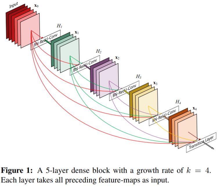
Dense connectivity

To further improve the information flow between layers we propose a different connectivity pattern: we introduce direct connections from any layer to all subsequent layers. Figure 1 illustrates the layout of the resulting DenseNet schematically. Consequently, the ℓth layer receives the feature-maps of all preceding layers, $x_0, \cdots, x_{l-1}$, as input:
$$
x_l=H_l([x_0,x_1,\cdots,x_{l-1}])
$$
where $[x_0,x_1,\cdots,x_{l-1}]$ refers to the concatenation of the feature-maps produced in layers $0, \cdots, l−1$.

Pooling layers

The concatenation operation used in Eq. (2) is not viable when the size of feature-maps changes. However, an essential part of convolutional networks is down-sampling layers that change the size of feature-maps. To facilitate down-sampling in our architecture we divide the network into multiple densely connected dense blocks; see Figure 2. We refer to layers between blocks as transition layers, which do convolution and pooling. The transition layers used in our experiments consist of a batch normalization layer and an $1\times 1$ convolutional layer followed by a $2\times 2$ average pooling layer.

Growth rate

If each function $H_l$ produces $k$ feature maps, it follows that the $l$-th layer has $k_0 + k\times (l−1)$ input feature-maps, where $k_0$ is the number of channels in the input layer. An important difference between DenseNet and existing network architectures is that DenseNet can have very narrow layers, e.g., $k = 12$. We refer to the hyperparameter $k$ as the growth rate of the network. We show in Section 4 that a relatively small growth rate is sufficient to obtain state-of-the-art results on the datasets that we tested on.

One explanation for this is that each layer has access to all the preceding feature-maps in its block and, therefore, to the network’s “collective knowledge”. One can view the feature-maps as the global state of the network. Each layer adds $k$ feature-maps of its own to this state. The growth rate regulates how much new information each layer contributes to the global state. The global state, once written, can be accessed from everywhere within the network and, unlike in traditional network architectures, there is no need to replicate it from layer to layer.

Bottleneck layers

Although each layer only produces $k$ output feature-maps, it typically has many more inputs. It has been noted in [36, 11] that a $1\times 1$ convolution can be introduced as bottleneck layer before each $3\times 3$ convolution to reduce the number of input feature-maps, and thus to improve computational efficiency. We find this design especially effective for DenseNet and we refer to our network with such a bottleneck layer, i.e., to the BN-ReLU-Conv($1\times 1$)-BN-ReLU-Conv($3\times 3$) version of $H_l$, as DenseNet-B. In our experiments, we let each $1\times 1$ convolution produce 4k feature-maps.

Identity Mappings in Deep Residual Networks

Paper: Identity mappings in deep residual networks

Introduction

ResNet已经成了很多CV任务的标配，作者Kaiming He在ResNet里引入了shortcut来辅助DCNN的学习与优化，但是对于shortcut为什么能work则没有过多提及。本文是ResNet作者本人发表在ECCV’16上的Paper，主要在于解释identical mapping为何能work，并且对比了identical mapping的一些变体，最后提出了pre-activation。

Delve Into ResNet and Identical Mapping

ResNet可以表示为这样：
$$
y_l=h(x_l) + \mathcal{F}(x_l,\mathcal{W}_l)
$$

$$
x_{l+1} = f(y_l)
$$
其中，$\mathcal{F}$代表residual function，$h(x_l)=x_l$代表identical mapping，$f$代表ReLU函数。

在本文中，作者发现，若$h(x_l)$和$f(y_l)$都是identical mapping的话，信息就可以直接从一个unit传播到下几层的units，无论是在forward还是backward都是如此。

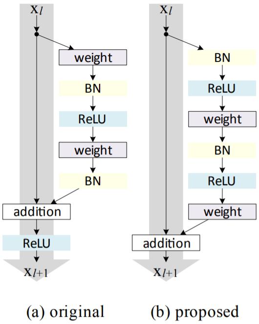
为了构造identical mapping $f(y_l)=y_l$，我们可以将activation function (ReLU and BN)看作weight layers的pre-activation。

Analysis of Deep Residual Networks

CVPR’15 Best Paper中的原始ResNet Unit是这样的：
$$
y_l=h(x_l)+\mathcal{F}(x_l, \mathcal{W}_l)
$$

$$
x_{l+1}=f(y_l)
$$
若$f$也是identical mapping: $x_{l+1}\equiv y_l$，就可以得到：
$$
x_{l+1}=x_l+\mathcal{F}(x_l,\mathcal{W}_l)
$$
Recursively，我们可以得到：
$$
x_{l+2}=x_{l+1}+\mathcal{F}(x_{l+1}, \mathcal{W}_{l+1})=x_l+\mathcal{F}(x_l, \mathcal{W}_l)+\mathcal{F}(x_{l+1}, \mathcal{W}_{l+1})
$$
所以有：
$$
x_L=x_l+\sum_{i=l}^{L-1}\mathcal{F}(x_i,\mathcal{W}_i)
$$
所以，对于deep的$L$层和shallow的$l$层，特征$x_L$可以表示成shallow unit feature $x_l$和residual function $\sum_{i=l}^{L-1}\mathcal{F}$的加和！说明：

1. 模型是任意units $L$和$l$ 的residual function
2. 特征$x_L=x_0+\sum_{i=0}^{L-1}\mathcal{F}(x_i,\mathcal{W}_i)$是所有proceeding residual functions输出的summation再加上$x_0$

BP的时候，根据chain rule，就得到如下公式(假设loss function为$\epsilon$)：
$$
\frac{\partial \epsilon}{\partial x_l}=\frac{\partial \epsilon}{\partial x_L}\frac{\partial x_L}{\partial x_l}=\frac{\partial \epsilon}{\partial x_L}(1+\frac{\partial }{\partial x_l} \sum_{i=l}^{L-1}\mathcal{F}(x_i,\mathcal{W}_i))
$$
所以，梯度$\frac{\partial \epsilon}{\partial x_l}$可以看作两个部分：

1. $\frac{\partial \epsilon}{\partial x_L}$直接从高层流通回来
2. $\frac{\partial \epsilon}{\partial x_L}(\frac{\partial }{\partial x_l}\sum_{i=l}^{L-1}\mathcal{F})$流经了其他的weight layers

Discussions

Paper里也对一些identical mapping的变体进行了实验与探讨，反正scaling, gating, $1\times 1$ convolutions, and dropout都效果不如原来的好。并且，由于$1\times 1$ conv引入了更多的参数，理论上讲representation learning ability是要比原来的ResNet要高的，结果却比原来低，说明这种performance drop不是因为representation ability，而是因为优化问题所致。

The shortcut connections are the most direct paths for the information to propagate. Multiplicative manipulations (scaling, gating, $1\times 1$ convolutions, and dropout) on the shortcuts can hamper information propagation and lead to optimization problems. It is noteworthy that the gating and $1\times 1$ convolutional shortcuts introduce more parameters, and should have stronger representational abilities than identity shortcuts. In fact, the shortcut-only gating and $1\times 1$ convolution cover the solution space of identity shortcuts (i.e., they could be optimized as identity shortcuts. However, their training error is higher than that of identity shortcuts,indicating that the degradation of these models is caused by optimization issues, instead of representational abilities.

此外，作者还验证了，当使用BN + ReLU作为pre-activation时，模型performance有了显著地改善。这种改善主要由两点带来：

1. 因为$f$是identical mapping，所以整个模型的optimization更容易了。
2. 使用BN作为pre-activation增加了模型的regularization，因BN本身具有regularization的效果。在CVPR’15原始版本的ResNet中，尽管BN normalize了信号，但是却立刻被添加进了shortcut，和未被BN normalize的signal一起merge了。而在pre-activation中，所有weight layers的input均被normalize了。

CliqueNet

Paper: Convolutional Neural Networks with Alternately Updated Clique

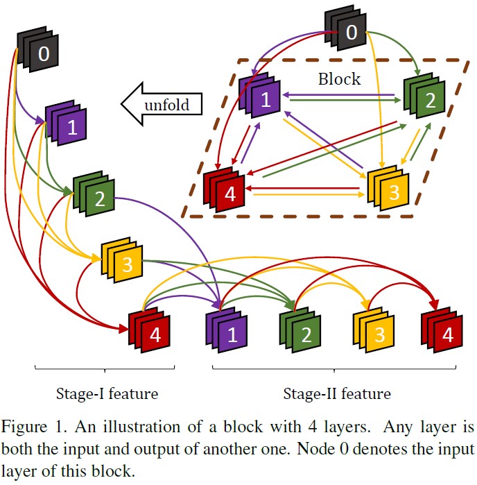
CliqueNet是发表在CVPR 2018上的Paper,在Deep CNN的设计方面又进了一步。前面我们已经谈到，自从ResNet/HighwayNet起，skip connection就被广泛应用于Deep Model的设计中（例如后来CVPR 2017的DenseNet）。在CliqueNet中，各个layer通过skip connection被设计成了环状结构(也就是说，在同一个block中，每一层既是其他layer的输入，也是其他layer的输出)，从而可以辅助更好的 information flow。新update的layers被concatenate来重新之前updated layers，参数被多次重用。因此这种recurrent结构能够将高层的information传递到低层，并且起到 spatial attention 的效果。而且通过使用multi-scale feature strategy，也可以避免产生过多的参数。CliqueNet的basic block如下：

What is CliqueNet?

前面已经提到了，skip connection现在俨然已成为CV/DCNN领域的神器，ResNet作者Kaiming He在最原始的ResNet中却对skip connection并未做过多的解释。所以最近的一些work中也有专门去分析shortcut的，有researcher认为ResNet可以看作是一系列小浅层网络的ensemble，也有人将skip connection解释为RNN/LSTM，在不同layers中weights被共享。

@LucasX注：如果读者有读过HighwayNet原文的话，就会深有体会了，是真的跟RNN很像啊。

Attention 也是在许多CV任务中被广泛应用的，其idea来源于人类的视觉系统，例如当人类在观察某样东西时，对当前眼睛里观察到的画面，注意力并非完全一致的，对某些物体总会施加过多的关注。而skip connection可以将高层语义信息带回到低层，并且可以re-weight这种focus，因此可以suppress一些背景/噪声信息，从而使得当前的feature map包含更多对分类更为discriminative的信息。

在CliqueNet中，信息是这样传递的：
前几层的feature map被concatenate来更新下一层，然后新update的层又被concatenate用来更新前面的层，因此information flow和feedback mechanism都可以被最大化。(读者可能有点绕，不太明白的话，可以看看上面那个图Clique Block，它是环状结构。)

CliqueNet有如下特性：

1. 参数少；DenseNet需要$C_n^2$个group的参数，CliqueNet需要$A_n^2$组。然而，DenseNet的filter数量随着depth增长而线性增长，所以DenseNet在网络结构过深时需要很多的参数。而在CliqueNet的每一个block中，只有Stage II的feature被feed到下一个block。此外，传统的网络新增了一层来做shortcut，而在CliqueNet中，weights被循环使用多次，所以当参数量固定的时候，可以获取deeper representation space。

CliqueNet Architecture

CliqueNet主要有两个重要组件：

• Clique Block: 来辅助feature的refinement
• Multi-scale Feature Strategy: 来保证参数的高效利用

CliqueNet的网络结构如下：

Clique Block

为了保证信息的高效流通，在CliqueNet中，相同block中除了input layer之外的任意两层都被双向连接（即该层既是其他层的输出，又是其他层的输入）。在Stage I，输入层$X_0$通过单向连接初始化该block的所有层，所有被updated layer都被concatenate来update下一层。在Stage II，layers开始选择性地update，除了top layer之外的所有层都被concatenate起来。因此，第$k (k\geq 2)$个loop中的第$i (i\geq 1)$层可以表示为：
$$
X_i^{(k)}=g(\sum_{l<i} W_{li}\star X_l^{(k)} + \sum_{m>i} W_{mi} \star X_m^{(k-1)})
$$

其中$\star$代表conv，权重$W_{ij}$在不同的stage保持重用。每一层都会接受来自最近更新的feedback information，这种top-down refinement可达到spatial attention mechanism的效果。

Feature at Different Stages

因为Stage II feature因attention得到了提纯，并且获取了更high-level的representation，我们将Stage II feature和input layer做concatenate作为block feature，然后走GAP后直接输入到loss layer，只有Stage II的feature被输入到下一个Clique Block中。通过这种方式，我们就获得了multi-scale feature representation，并且每一个block的dimensionality不会增长过大。

Extra Techniques

除了上述的两个main components，作者也使用了一些其他的tricks来刷分。

Attention transition

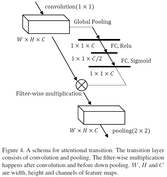
CliqueNet使用high level visual information来refine low level activations。Attention mechanism通过对feature map进行加权，来弱化noise和background。在CliqueNet中，filters在transition的conv layer之后进行global average，然后接两层FC layers。第一个FC layer使用ReLU和一半数量的filters，第二个FC layer使用sigmoid和相同数量的filters。因此activation被归一化到$[0, 1]$区间，并且通过filter-wise multiplication作为input。

Bottleneck and compression

We introduce bottleneck to our large models. The $3\times 3$ convolution kernels in each block are replaced by $1\times 1$, and produce a middle layer, after which, a $3\times 3$ convolution layer follows to produce the top layer. The middle layer and top layer contain the same number of feature maps. Compression is another tool adopted in [17] to make the model more compact. Instead of compressing the number of filters in transition layers as they do, we only compress the features that are accessed to the loss function, i.e. the Stage-II concatenated with its input layer. The models with compression have an extra convolutional layer with $1\times 1$ kernel size before global pooling. It generates half the number of filters to enhance model compactness and keep the dimensionality of the final feature in a proper range.

Further Discussion

• Parameter efficiency
  因为multi-scale feature strategy仅仅将Stage-II feature transit到下一个block（而不是像DenseNet那样stack feature map到更深的层）。

• Feature refinement

  In CliqueNet, the layers are updated alternately so that they are supervised by each other. Moreover, in the second stage, feature maps always receive a higher-level information from the filters that are updated more lately. This spatial attention mechanism makes layers refined repeatedly, and is able to repress the noises or background of images and focus more activations on the region that characterize the target object. In order to test the effects, we visualize the feature maps following the methods in [43]. As shown in Figure 6, we choose three input images with complex background from ImageNet validation set, and visualize their feature maps with the highest average activation magnitude in the Stage-I and Stage-II, respectively. It is observed that, compared with the Stage-I, the feature maps in Stage-II diminish the activations of surrounding objects and focus more attention on the target region. This is in line with the conclusion in Table 2 that the Stage-II feature is more discriminative and leads to a better performance.

  

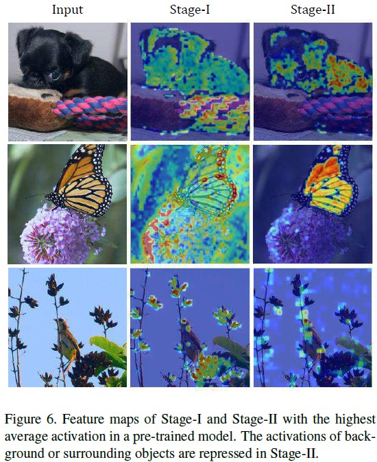
  可以看到，对Feature activation做可视化之后，Stage-II相比较于Stage-I，明显削弱了一些背景信息，从而使得object主体信息更加明显，进而有助于提升分类性能。

PeleeNet

Paper: Pelee: A Real-Time Object Detection System on Mobile Devices

提起DNN for Mobile/Efficiency Architecture，Depth-wise Convolution自然不会陌生，我们前面也讲到过ShuffleNet/MobileNet这些专为移动端设计的网络结构。本文介绍一篇来自NeurIPS2018上的高性能网络结构——PeleeNet。

传统的移动端高效网络结构往往依赖于DW Separable Conv，但是在现如今绝大多数的Deep Learning Framework(例如TensorFlow/PyTorch等)却缺乏对DW Separable Conv的高效实现，因此PeleeNet是完全基于传统卷积而设计的。也就是说，要设计高效的网络结构，也不一定非得靠DW Conv嘛~

Details of PeleeNet

PeleeNet的设计主要idea如下：

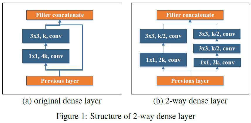
• Two-way Dense Layer: 这一点idea来源于GoogLeNet，PeleeNet使用这种结构来获取不同尺度的receptive fields。一种way使用$3\times 3$ kernel size；另一种使用堆叠的两个$3\times 3$ conv来学习larger objects的feature。结构如下：
  
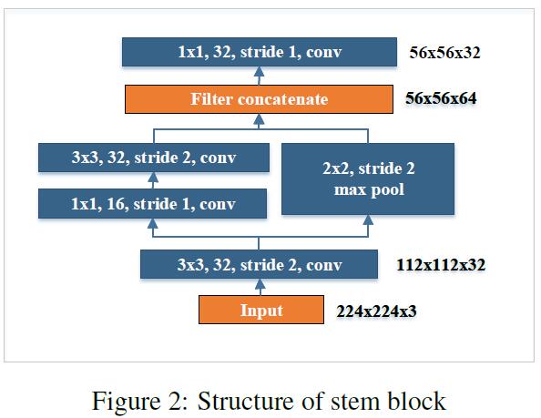
• Stem Block: 在第一个dense layer之前加入了stem block，可以做到在增强feature representation ability的同时不引入过多的computational burden，这种方法比现如今主流方法(例如增加feature map的channel数量，增加depth)要更优越。
  
• Dynamic Number of Channels in Bottleneck Layer: 简而言之，bottleneck layers中channel的数量是随着输入尺寸而变动的。而不像DenseNet中采用固定的4倍layers增长速率。
• Transition Layer Without Compression: 作者在实验中发现，DenseNet提出的compression factor会损害feature representation ability。因此PeleeNet的transition layers中，output channels数量总是和input channels数量保持一致。
• Composite Function: 作者采用post-activation来进一步加速网络。在预测阶段，所有的BN layers都可以被merge进conv layers，从而大幅提升效率。为了抵消这种post-activation带来的不良影响，我们使用了shallow and wide structure。此外，作者在最后一个dense block之后还使用了一个额外的$1\times 1$ conv layer来进一步加强整个网络的非线性能力，从而提升representation learning ability。

此外，为了在detection任务中获得性能提升，作者将PeleeNet融合进了SSD，并且做了如下改进：

• Feature Map Selection: 为了加速，作者没有使用$38\times 38$的feature map，而是使用了这5个multi-scale的feature map: $19\times 19$, $10\times 10$, $5\times 5$, $3\times 3$以及 $1\times 1$。
• Residual Prediction Block: 对于每个将被应用到detection的feature map，都先走一遍residual block。
  
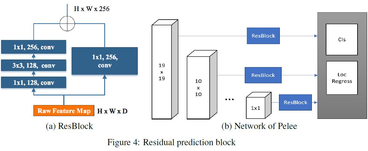
• Small Conv Kernel for Prediction: 作者在实验中发现，使用$1\times 1$ conv和$3\times 3$ conv做预测时accuracy几乎一样，但是却可以带来很大的速度提升。

Ablation Study

作者在train ImageNet任务时，使用了Cosine Learning Rate Annealing的策略：
$$
0.5\times lr\times(cos(\pi \times t/120) + 1)
$$

为了加速deep model的inference time，一个惯用做法是使用FP16来代替FP32。然而，由DW Separable Conv设计而来的网络结构很难从FP16 inference engine中获得提升。作者观察到使用FP16的MobileNet V2和使用FP32的MobileNet V2速度几乎一致。

SENet

Paper: Squeeze-and-Excitation Networks

CNN驱动了很多视觉任务的发展，我们可以看到，从最初的AlexNet到DenseNet/CliqueNet，网络结构的设计方面也是越来越精巧。本文介绍CVPR 2018上的一篇Paper——SENet。

SENet主要关注的是channel relationship，通过Squeeze-and-Excitation Unit可以做到feature recalibration，即利用global information来使得feature maps中more informative的feature得到关注，less useful的feature得到抑制(是不是有点Attention的意思?)。

SE Block可以表示如下：对于任意一种变换$F_{tr}: X\to U,X\in \mathbb{R}^{H^{‘}\times W^{‘}\times C^{‘}}, U\in \mathbb{R}^{H\times W\times C}$，我们可以利用SE Block来进行feature recalibration:
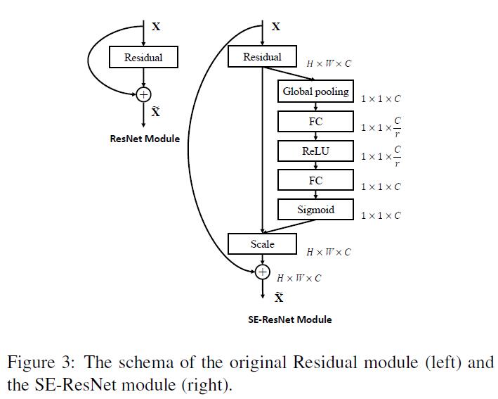
feature $U$首先经过 squeeze operation，来将跨spatial dimension的feature maps进行aggregation，来产生channel descriptor。因该channel descriptor包含了channel-wise feature response的global distribution信息，所以可以让lower layers利用global receptive fields的信息。在该步骤之后，会经历 excitation operation，即每一个channel通过 self-gating mechanism 学习到的sample-specific activation，来掌握自己的excitation。然后feature map $U$ 被重新赋予不同的权重以产生SE Block最终的输出。整体示意图如下：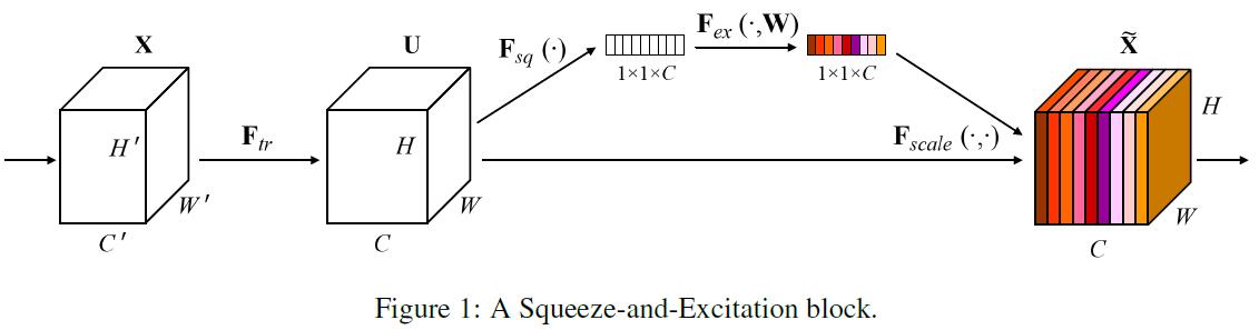

Group Convolution可以被用来增加cardinality(即transformation的数量)，读者如果对ResNeXt有印象的话，此处应该不会陌生了。Multi-branch可以被视为group convolution的一种，它可以得到更加flexible的operator composition。

Cross-channel Correlation可以看作是feature的重新组合(读者不妨回忆一下DW Separable Convolution)，SE Unit中，non-linearity dependencies利用global information可以使得学习更加容易，并且极大地提升网络的表示能力。

Attention and Gating Mechanism

Attention can be viewed, broadly, as a tool to bias the allocation of available processing resources towards the most informative components of an input signal [17, 18, 22, 29, 32]. The benefits of such a mechanism have been shown across a range of tasks, from localisation and understanding in images [3, 19] to sequence-based models [2, 28]. It is typically implemented in combination with a gating function (e.g. a softmax or sigmoid) and sequential techniques [12, 41].

In contrast, our proposed SE block is a lightweight gating mechanism, specialised to model channel-wise relationships in a computationally efficient manner and designed to enhance the representational power of basic modules throughout the network.

Squeeze-and-Excitation Blocks

SE Block是一种可完成如下变换的计算单元：$F_{tr}: X\to U,X\in \mathbb{R}^{H^{‘}\times W^{‘}\times C^{‘}}, U\in \mathbb{R}^{H\times W\times C}$。设$V=[v_1,v_2,\cdots,v_C]$代表学习的filters。我们将$F_{tr}$的输出重写为$U=[u_1,u_2,\cdots,u_C]$:
$$
u_c=v_c\star X=\sum_{s=1}^{C^{‘}}v_c^s\star x^s
$$
$\star$代表卷积操作，$v_c^s$是2D spatial kernel，因此代表单通道$v_c$作用在$X$对应的channel上。因输出是所有channels的summation，所以channel dependencies被隐式地包含进了$v_c$。

Squeeze: Global Information Embedding

In order to tackle the issue of exploiting channel dependencies, we first consider the signal to each channel in the output features. Each of the learned filters operates with a local receptive field and consequently each unit of the transformation output $U$ is unable to exploit contextual information outside of this region. This is an issue that becomes more severe in the lower layers of the network whose receptive field sizes are small.

To mitigate this problem, we propose to squeeze global spatial information into a channel descriptor. This is achieved by using global average pooling to generate channel-wise statistics. Formally, a statistic $z\in \mathbb{R}^C$ is generated by shrinking $U$ through spatial dimensions $H\times W$, where the $c$-th element of $z$ is calculated by:
$$
z_c=F_{sq}(u_c)=\frac{1}{H\times W}\sum_{i=1}^H \sum_{j=1}^Wu_c(i, j)
$$

The transformation output U can be interpreted as a collection of the local descriptors whose statistics are expressive for the whole image. Exploiting such information is prevalent in feature engineering work [35, 38, 49]. We opt for the simplest, global average pooling, noting that more sophisticated aggregation strategies could be employed here as well.

Excitation: Adaptive Recalibration

To make use of the information aggregated in the squeeze operation, we follow it with a second operation which aims to fully capture channel-wise dependencies. To fulfil this objective, the function must meet two criteria: first, it must be flexible (in particular, it must be capable of learning a nonlinear interaction between channels) and second, it must learn a non-mutually-exclusive relationship since we would like to ensure that multiple channels are allowed to be emphasised opposed to one-hot activation. To meet these criteria, we opt to employ a simple gating mechanism with a sigmoid activation:
$$
s=F_{ex}(z, W)=\sigma(g(z,W))=\sigma(W_2 \delta(W_1z))
$$
$\delta$代表ReLU，$W_1\in \mathbb{R}^{\frac{C}{r}\times C}$，$W_2\in \mathbb{R}^{C\times \frac{C}{r}}$。为了限制模型复杂度以及辅助泛化能力，我们在non-linearity(例如带reduction ratio $r$的dimension-reduction layer$W_1$)周围通过构建2层fully connected layers的bottleneck来参数化gating mechanism。SE Block最终的输出通过rescale transformation output $U$ with activations得到:
$$
\tilde{x}_c=F_{scale}(u_c,s_c)=s_c\cdot u_c
$$
其中，$\tilde{X}=[\tilde{x}_1,\tilde{x}_2,\cdots,\tilde{x}_C]$，$F_{scale}(u_c,s_c)$代表channel-wise multiplication between feature map $u_c\in \mathbb{R}^{H\times W}$ and scalar $s_c$。

The activations act as channel weights adapted to the input-specific descriptor $z$. In this regard, SE blocks intrinsically introduce dynamics conditioned on the input, helping to boost feature discriminability.

此外，还可以将SE Unit融合进当前mainstream的DCNN中：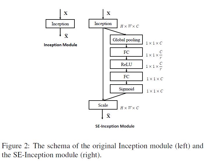

Slimmable Neural Network

Paper: Slimmable Neural Network

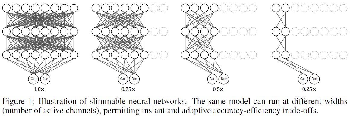
近年来，深度学习的火热驱动了越来越多任务性能的大幅提升，尤其是在CV，从AlexNet到CliqueNet，网络结构越来越精巧。此外，针对移动端的网络结构设计(如MobileNet/ShuffleNet/PeleeNet等)也得到了非常多的关注。但是，即便是专门为移动端设计的网络结构，也是不能通用的。例如Android设备的碎片化问题，以及同一部手机在不同时间段内后台任务对资源的占用率问题。

针对以上问题，作者设计了switchable batch normalization，在测试时，网络可以根据当前设备的resource constraints来自动调整width来保证accuracy和latency的tradeoff。

SNN有以下好处：

1. 对于不同的环境，我们只需要训练单个模型。
2. 在target device上可以根据device本身的computational constraint自动调整active channels。
3. SNN可以应用到各种结构的网络中(FC/Conv/DW Conv/Group Conv/Dilated Conv)和各种不同的应用(Classification/Detection/Segmentation)中。
4. 当Switch到不同configuration时，SNN的运行不需要额外的runtime和memory cost。

Empirically training neural networks with multiple switches has an extremely low testing accuracy around 0.1% for 1000-class ImageNet classification. We conjecture it is mainly due to the problem that accumulating different number of channels results in different feature mean and variance. This discrepancy of feature mean and variance across different switches leads to inaccurate statistics of shared Batch Normalization layers (Ioffe & Szegedy, 2015), an important training stabilizer. To this end, we propose a simple and effective approach, switchable batch normalization, that privatizes batch normalization for different switches of a slimmable network. The variables of moving averaged means and variances can independently accumulate feature statistics of each switch. Moreover, Batch Normalization usually comes with two additional learnable scale and bias parameter to ensure same representation space (Ioffe & Szegedy, 2015). These two parameters may able to act as conditional parameters for different switches, since the computation graph of a slimmable network depends on the width configuration. It is noteworthy that the scale and bias can be merged into variables of moving mean and variance after training, thus by default we also use independent scale and bias as they come for free. Importantly, batch normalization layers usually have negligible size (less than 1%) in a model.

Details of Slimmable Neural Network

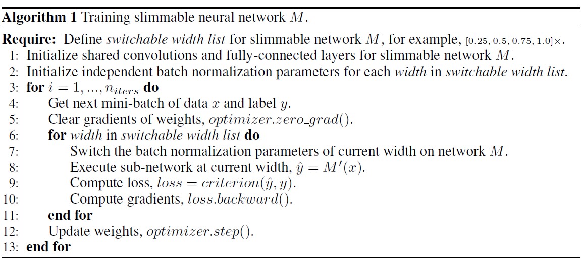
To train slimmable neural networks, we begin with a naive approach, where we directly train a shared neural network with different width configurations. The training framework is similar to the one of our final approach, as shown in Algorithm 1. The training is stable, however, the network obtains extremely low top-1 testing accuracy around 0.1% on 1000-class ImageNet classification. We conjecture the major problem in the naive approach is that: for a single channel in a layer, different numbers of input channels in previous layer result in different means and variances of the aggregated feature, which are then rolling averaged to a shared batch normalization layer. The inconsistency leads to inaccurate batch normalization statistics in a layer-by-layer propagating manner. Note that these batch normalization statistics (moving averaged means and variances) are only used during testing, in training the means and variances of the current mini-batch are used.

作者在实验中证明，先train base-net——A，再添加额外参数B来形成新的模型A+B (MobileNet V2 0.5×)只会带来非常微小的performance boost(from 60.3% to 61.0%)。但单独train一个A+B (MobileNet V2 0.5×)会提升到65.4%。这是因为将B添加到A之后，会引入新的connection (A-B, B-B, B-A)，而这种incremental training会抑制A和B权重的joint adaption。

We then investigate incremental training approach (a.k.a. progressive training). We first train a base model A (MobileNet v2 0.35×). We fix it and add extra parameters B to make it an extended model A+B (MobileNet v2 0.5×). The extra parameters are fine-tuned along with the fixed parameters of A on the training data. Although the approach is stable in both training and testing, the top-1 accuracy only increases from 60.3% of A to 61.0% of A+B. In contrast, individually trained MobileNet v2 0.5× achieves 65.4% accuracy on the ImageNet validation set. The major reason for this accuracy degradation is that when expanding base model A to the next level A+B, new connections, not only from B to B, but also from B to A and from A to B, are added in the computation graph. The incremental training prohibits joint adaptation of weights A and B, significantly deteriorating the overall performance.

Switchable Batch Normalization

Motivated by the investigations above, we present a simple and highly effective approach, named Switchable Batch Normalization (S-BN), that employs independent batch normalization (Ioffe & Szegedy, 2015) for different switches in a slimmable network. Batch normalization (BN) was originally proposed to reduce internal covariate shift by normalizing the feature: $y^{‘}=\gamma\frac{y-\mu}{\sqrt{\sigma^2+\epsilon}}+\beta$.
where $y$ is the input to be normalized and $y^{‘}$ is the output, $\gamma, \beta$ are learnable scale and bias, $\mu$, $\sigma^2$ are mean and variance of current mini-batch during training. During testing, moving averaged statistics of means and variances across all training images are used instead. BN enables faster and stabler training of deep neural networks (Ioffe & Szegedy, 2015; Radford et al., 2015), also it can encode conditional information to feature representations (Perez et al., 2017b; Li et al., 2016b).

To train slimmable networks, S-BN privatizes all batch normalization layers for each switch in a slimmable network. Compared with the naive training approach, it solves the problem of feature aggregation inconsistency between different switches by independently normalizing the feature mean and variance during testing. The scale and bias in S-BN may be able to encode conditional information of width configuration of current switch (the scale and bias can be merged into variables of moving mean and variance after training, thus by default we also use independent scale and bias as they come for free). Moreover, in contrast to incremental training, with S-BN we can jointly train all switches at different widths, therefore all weights are jointly updated to achieve a better performance.

S-BN also has two important advantages:

1. The number of extra parameters is negligible.
2. The runtime overhead is also negligible for deployment. In practice, batch normalization layers are typically fused into convolution layers for efficient inference. For slimmable networks, the re-fusing of batch normalization can be done on the fly at runtime since its time cost is negligible. After switching to a new configuration, the slimmable network becomes a normal network to run without additional runtime and memory cost.

Training of SNN

Our primary objective to train a slimmable neural network is to optimize its accuracy averaged from all switches. Thus, we compute the loss of the model by taking an un-weighted sum of all training losses of different switches. Algorithm 1 illustrates a memory-efficient implementation of the training framework, which is straightforward to integrate into current neural network libraries. The switchable width list is predefined, indicating the available switches in a slimmable network. During training, we accumulate back-propagated gradients of all switches, and update weights afterwards.

MixNet

Paper: “MixNet: Mixed Depthwise Convolutional Kernels.”
Code: MixNet.TF

MixNet是Google发表在BMVC19上的文章，核心idea其实也非常简单。个人理解，就是将GoogLeNet中利用multi-size kernel设计Inception Block来获取multi-scale feature的思路用在了Depth-wise Conv上。

作者首先分析了large scale对模型性能的影响：随着kernel size的增加，model size自然也随之增加，从$3\times 3$增加到$7\times 7$时，Acc也逐步增加，但是当kernel size大于$9\times 9$时则Acc会急剧下降，说明太大的kernel size会hurt模型的性能。同时，在MobileNet V1结构中，$7\times 7$取得最佳效果，而MobileNet V2中，$9\times 9$取得最佳效果。作者还意识到：single kernel size会有局限性，因此需要在网络中同时使用large kernel来capture high-resolution patterns，同时small kernels来capture low-resolution patterns，才能获得更好的Acc与efficiency。这也就是本文MixNet的初衷。

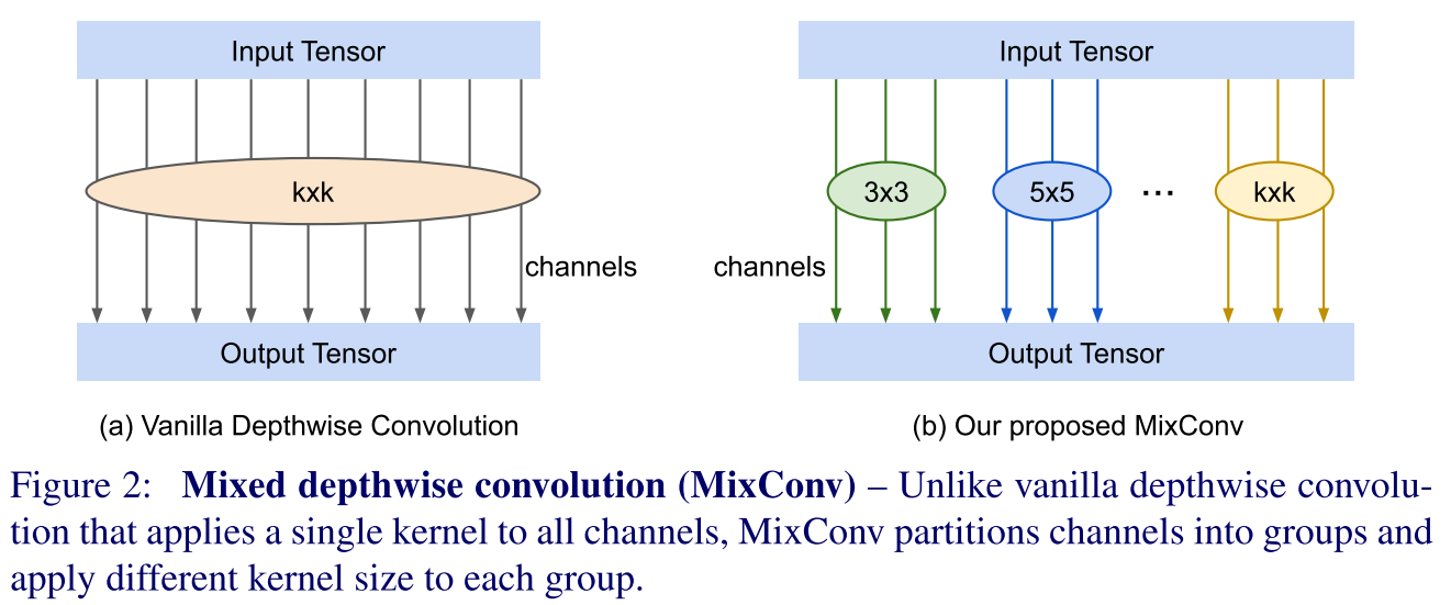
MixConv首先将channels进行分组，并且为不同的组分配不同的conv kernel size来capture不同的patterns，这样就得到了学习了不同pattern的features：$<\hat{Y}_{x,y,z_1}^1,\cdots,\hat{Y}_{x,y,z_g}^g>$。接下来将这些features进行concatenate操作即可获得最终的feature representation：
$$
Y_{x,y,z_0}=Concat(\hat{Y}_{x,y,z_1}^1,\cdots,\hat{Y}_{x,y,z_g}^g)
$$

核心idea就是这么简单，作者在实验中也将这种思路分别用在了hand-crafted architecture与NAS中，发现均取得了很好地效果。

SKNet

Paper: Selective Kernel Networks
Code: SKNet.Caffe

SKNet是发表在CVPR’19上的paper，是手工设计网络的进一步进展（笔者认为，现如今其实SENet在图像分类这个任务上已经做得足够好了），idea也非常简单，主体思路和Inception比较类似，就是如何获取multi-scale information。

Paper开篇，作者先引用了神经学领域的一些工作来作为引子，引出Receptive Fields size实际上并不是一样的（PS：这一招可以学一学，增强文章逼格）。提到multi-scale information，就不得不提Inception网络了，因为Inception Block也是通过设计不同size的conv filter来处理multi-scale信息，但是处理完之后，Inception只是单纯的做linear aggregation，所以不一定能获取最佳的adaption ability。

SK Unit一共由3个部分组成：

• Split: 和Inception类似，multi-branch结构，设置不同size的conv filter，来获取multi-scale的信息。
• Fuse: 对来自不同branch的multi-scale信息进行整合
• Select: 根据selection weights重新对信息进行加权，即Attention，和SENet类似

Selective Kernel Convolution

Split

对于feature map $X\in \mathbb{R}^{H^{‘}\times W^{‘}\times C^{‘}}$，经过两种transformations: $\tilde{\mathcal{F}}: X\rightarrow \tilde{U}\in \mathbb{R}^{H\times W\times C}$，以及$\hat{\mathcal{F}}: X\rightarrow \hat{U}\in \mathbb{R}^{H\times W\times C}$，前者kernel size为3，后者kernel size为5。为了进一步减小参数量，$5\times 5$ kernel由$stride=2$的$3\times 3$ dilatetion conv代替。

Fuse

先对上一步Split的两个branch信息进行Elt-wise summation:
$$
U=\tilde{U} + \hat{U}
$$
然后通过Global Average Pooling来embed global information，这个时候就得到了channel-wise statistics向量$s\in \mathbb{R}^C$，其中$s$向量中第$c$维的计算方式为:
$$
s_c=\mathcal{F}_{gap}(U_c)=\frac{1}{H\times W}\sum_{i=1}^H \sum_{j=1}^W U_c(i,j)
$$
紧接着再跟一个Fully connected layers来得到$z\in \mathbb{R}^{d\times 1}$，其中$d<C$，起到降维的作用。
$$
z=\mathcal{F}_{fc}(s)=\delta(\mathcal{B}(Ws))
$$
其中$\delta$是ReLU，$\mathcal{B}$是BatchNorm。为了研究$d$对模型efficiency的影响，作者在这里引入了参数$r$来控制$d$的值:
$$
d=max(C/r, L)
$$

Select

和SENet类似，cross-channel的soft attention用于选择不同spatial scale的信息:
$$
a_c=\frac{e^{A_c z}}{e^{A_c z} + e^{B_c z}}
$$

$$
b_c=\frac{e^{B_c z}}{e^{A_c z} + e^{B_c z}}
$$
其中$A,B\in \mathbb{R}^{C\times d}$，$a$和$b$分别代表$\tilde{U}$和$\hat{U}$的soft attention向量。经过attention加权，最终的feature map $V$为:
$$
V_c=a_c\cdot \tilde{U}_c + b_c\cdot \hat{U}_c
$$
其中$a_c+b_c=1$。

SKNet的整体网络结构如下：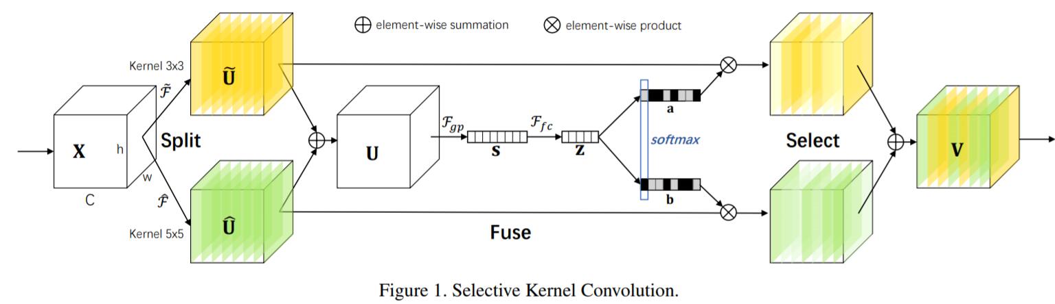

此外，作者在实验中发现，target object越大，该object就得到越强的attention。

Reference

1. Krizhevsky A, Sutskever I, Hinton G E. Imagenet classification with deep convolutional neural networks[C]//Advances in neural information processing systems. 2012: 1097-1105.
2. Simonyan K, Zisserman A. Very deep convolutional networks for large-scale image recognition[J]. arXiv preprint arXiv:1409.1556, 2014.
3. Lin M, Chen Q, Yan S. Network in network[J]. arXiv preprint arXiv:1312.4400, 2013.
4. He K, Zhang X, Ren S, Sun J. Deep residual learning for image recognition. InProceedings of the IEEE conference on computer vision and pattern recognition 2016 (pp. 770-778).
5. Zhang, Xiangyu and Zhou, Xinyu and Lin, Mengxiao and Sun, Jian. ShuffleNet: An Extremely Efficient Convolutional Neural Network for Mobile Devices[C]//The IEEE Conference on Computer Vision and Pattern Recognition (CVPR). 2018
6. Chollet, Francois. “Xception: Deep Learning with Depthwise Separable Convolutions.” 2017 IEEE Conference on Computer Vision and Pattern Recognition (CVPR). IEEE, 2017.
7. Howard, Andrew G., et al. “Mobilenets: Efficient convolutional neural networks for mobile vision applications.” arXiv preprint arXiv:1704.04861 (2017).
8. Zhu, Mark Sandler Andrew Howard Menglong, and Andrey Zhmoginov Liang-Chieh Chen. “MobileNetV2: Inverted Residuals and Linear Bottlenecks.”[C]//The IEEE Conference on Computer Vision and Pattern Recognition (CVPR). 2018
9. Xie, Saining, et al. “Aggregated residual transformations for deep neural networks.” Computer Vision and Pattern Recognition (CVPR), 2017 IEEE Conference on. IEEE, 2017.
10. Huang, Gao, et al. “Densely Connected Convolutional Networks.” CVPR. Vol. 1. No. 2. 2017.
11. He K, Zhang X, Ren S, et al. Identity mappings in deep residual networks[C]//European conference on computer vision. Springer, Cham, 2016: 630-645.
12. Szegedy, Christian, et al. “Going deeper with convolutions.” Proceedings of the IEEE conference on computer vision and pattern recognition. 2015.
13. Yang Y, Zhong Z, Shen T, et al. Convolutional Neural Networks with Alternately Updated Clique[C]//Proceedings of the IEEE Conference on Computer Vision and Pattern Recognition. 2018: 2413-2422.
14. Zilly J G, Srivastava R K, Koutnı́k J, et al. Recurrent Highway Networks[C]//International Conference on Machine Learning. 2017: 4189-4198.
15. Wang, Jun and Bohn, Tanner and Ling, Charles. Pelee: A Real-Time Object Detection System on Mobile Devices[C]//Advances in Neural Information Processing Systems 31. 2018:1967–1976.
16. Hu, Jie and Shen, Li and Sun, Gang. Squeeze-and-Excitation Networks[C]//The IEEE Conference on Computer Vision and Pattern Recognition (CVPR). 2018.
17. Yu, Jiahui, et al. “Slimmable Neural Networks.”[C]//ICLR (2019).
18. Szegedy, Christian, et al. “Rethinking the inception architecture for computer vision.” Proceedings of the IEEE conference on computer vision and pattern recognition. 2016.
19. Tan, Mingxing, and Quoc V. Le. “MixNet: Mixed Depthwise Convolutional Kernels.” BMVC (2019).
20. Li X, Wang W, Hu X, et al. Selective Kernel Networks[C]//Proceedings of the IEEE Conference on Computer Vision and Pattern Recognition. 2019: 510-519.