[CV] Counting

Introduction

Counting是近年来CV领域一个受到关注越来越多的方向，它主要的应用场景就是密集场景下的人流估计、车辆估计等。近年来非常火热的新零售、智慧安防都有Counting的应用场景。Counting大体上可以分为两种方案，一种是基于detection的方式：即数bbox；另一种是直接回归density map的方式：即将counting问题转化为一个regression问题。基于detection的方法在目标非常密集的场景下就不适合了，所以在这种场景下density map regression还是目前的mainstream。

Counting的Metric通常为MAE和MSE，MAE评判counting heads的accuracy，MSE评判robustness。

@LucasXU注：本文长期更新。

Multi-Column CNN

Paper: Single-image crowd counting via multi-column convolutional neural network

MCNN (Multi-Column CNN)主要idea来自于2012年上的一篇CVPR Paper Multi-column Deep Neural Networks for Image Classification，什么叫multi-column呢？意思就是给定一张图，分3个并行的branch，每个branch采用不同的conv size/pooling stride等，最后用$1\times 1$ conv对这3个不同branch输出的feature map做linear weighted combination。注：Counting属于content geometry-sensitive task，一般不直接warp到fixed size。

MCNN有以下好处：

• 通过3个receptive fields不同(small/medium/large)column，每个column可以更好地适应由不同图像分辨率带来的不同尺度问题。
• 在MCNN中，作者将最后一层的FC替换为了$1\times 1$的conv layer，因此input image可以为任意尺寸，而不需要强行warp导致变形。网络的输出就是density estimate。

Delve into MCNN

Density map based crowd counting

通过DCNN来进行crowd counting主要有以下两种思路：第一种是直接回归(输入image，输出counting number)；第二种是输出crowd的density map(即每一平米有多少head count)，然后通过integration的方式进行head count计算。MCNN选用了第二种方式(即基于density map)，这样做有如下优点：

• Density map保留了更多的信息；与直接regress head count相比，density map保留了input image中crowd的spatial distribution，而这种spatial distribution information在很多任务中都是非常有用的。例如某个small region的density比其他regions要高很多，那么就可以说明这个region出现了something abnormal。
• 通过CNN学习density map，learned filters可以更好地适应于不同size的human head(因为实际场景中因拍摄角度、距离等因素，会造成人头尺寸在图片中不同的大小)，因此这些learned filters会更加semantic meaningful，进而提高整个模型的performance。

若pixel $x_i$有head，我们将其表示为一个函数$\delta(x-x_i)$，因此有$N$个labeled head的图片可以表示为：
$$
H(x)=\sum_{i=1}^N \delta(x-x_i)
$$

为了将其转换为一个连续密度函数，我们使用Gaussian Kernel $G_{\sigma}$来对$H(x)$进行卷积，所以density就成了$F(x)=H(x)\star G_{\sigma}(x)$。然而，这样的density function需要假定在图像空间中$x_i$都是互相独立的。这显然是不太符合实际的，实际上，每个$x_i$都是3D scene中因perspective distortion带来的crowd density的一个样本，并且这些pixels和scene中对应不同size的样本$x_i$都是有关联的。

因此，为了准确地预估crowd density $F$，我们需要考虑因ground plane和image plane的之间的homography带来的distortion问题。但是对于图片数据本身而言，我们并无法知道geometry scene是怎样的。然而，若我们假设每个head周围的crowd都是evenly distributed，那么这些head和其k近邻的平均距离就可以得到关于geometry distortion合理的预估。

因此，我们需要根据图片中每个person head的size来确定spread parameter $\sigma$。但现实中很难精确知道head size的大小，以及head size和density map的关系。作者发现，head size is relative to the distance between the centers of two neighboring persons in crowd scene。因此对于这些crowded scene的density map，可基于每个person head与其k近邻的平均距离来adaptively determine spread parameter。

对于图片中的每个head $x_i$，我们定义其k近邻为$\{d_1^i,d_2^i,\cdots,d_m^i\}$，平均距离为$\bar{d^i}=\frac{1}{m}\sum_{j=1}^m d_j^i$。因此，和$x_i$相关像素所对应在scene ground中的区域，与$\bar{d^i}$大致成半径比例。因此，为了估计pixel $x_i$周围的crowd density，我们用以与$\bar{d^i}$成比例的$\sigma_i$为variance的Gaussian Kernel去对$\delta(x-x_i)$进行卷积。Density $F$为：
$$
F(x)=\sum_{i=1}^N \delta(x-x_i)\star G_{\sigma_i}(x), \sigma_i=\beta \bar{d^i}
$$

for some parameter $\beta$. In other words, we convolve the labels $H$ with density kernels adaptive to the local geometry around each data point, referred to as geometry-adaptive kernels.

Multi column CNN for density map estimation

因perspective distortion，图片通常会包含各种不同size的head，因此不同receptive fields的conv filter能够capture到不同scale的crowd density。对应large receptive fields的conv filter对于estimate large head size的crowd更有用。

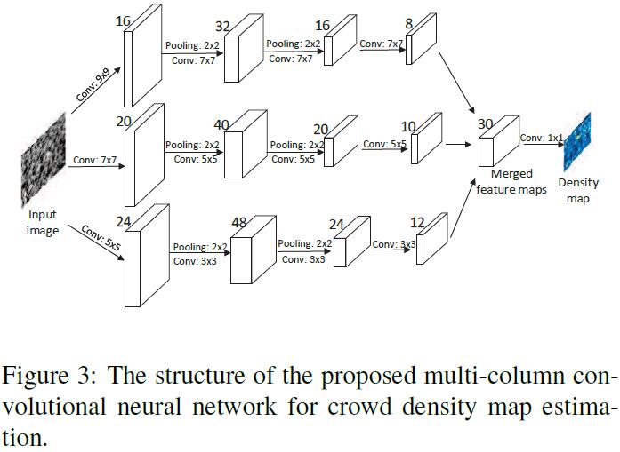
那么如何将feature map映射到density map呢？
作者是这样做的：将CNN所有的output feature maps堆叠起来，并使用$1\times 1$进行conv(实际上就是linear weighted combination；这个方法和Point-wise Convolution比较类似)。然后用Euclidean distance来measure estimated density map和groundtruth之间的difference。
$$
L(\Theta)=\frac{1}{2N}\sum_{i=1}^N|F(X_i;\Theta)-F_i|_2^2
$$

有这样一些data tricks值得mention一下：

• 传统CNN往往会normalize input来得到fixed size image，但是MCNN支持arbitrary size的input。因为resize会带来density map中的distortion问题，而这对于crowd density estimate是非常不利的。
• 和传统Multi-column粗暴地将feature map进行average相比，MCNN通过$1\times 1$ conv对其进行linear weighted combination。
• 在实验中，作者先单独pre-train 每个column，然后再将3个column进行fine-tune。

Leveraging Unlabeled Data for Crowd Counting by Learning to Rank

Paper: Leveraging Unlabeled Data for Crowd Counting by Learning to Rank

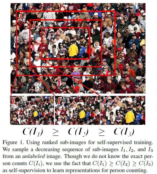
这篇文章将counting问题转化为了一个ranking问题，主要idea就是说在一张图中，crop下来的部分中包含的crowd number是肯定要不多于原图的crowd number。然后利用这个作为supervision signal，将其转化成为ranking问题。这样做就可以用到大量未标注crowd density的图片来做self supervised learning。

Counting近些年来得到了很大的关注，但是给这些人群密集的图片打label是非常麻烦的。最近self-supervised learning得到了越来越多的关注，它可以从auxiliary task(different but related to original supervised task)中进行学习。

本文提出的Learning to rank主要基于这样一个idea：尽管我们没办法获知一张crowd image中精确的crowd number，但是可以确定的是，crop samples from a crowd image contain the same or fewer persons than the original。这样我们就可以产生一系列sub-images的ranking，去训练网络预估一张图是否比另一张图包含更多的persons。

Generating ranked image sets for counting

• Input: A crowd scene image, number of patches $k$ and scale factor $s$.
• A list of patches ordered according to the number of persons in the patch.

Step 1: Choose an anchor point randomly from the anchor region. The anchor region is defined to be $1/r$ the size of the original image, centered at the original image center, and with the same aspect ratio as the original image.

Step 2: Find the largest square patch centered at the anchor point and contained within the image boundaries.

Step 3: Crop $k−1$ additional square patches, reducing size iteratively by a scale factor s. Keep all patches centered at anchor point.

Step 4: Resize all $k$ patches to input size of network.

Learning from ranked image sets

Crowd density estimation network

作者使用VGG16作为backbone network来回归crowd density map，但是去掉了两个fully connected layers和pool5来保留住更多的spatial resolution，并且增加了一个$3\times 3\times 512$和zero padding来保证same size。这里直接使用Euclidean distance来作为loss：
$$
L_{c}=\frac{1}{M}\sum_{i=1}^M (y_i-\hat{y}_i)^2
$$
$y_i$是groundtruth person density map，$\hat{y}_i$是prediction。

Crowd counting的groundtruth通常包含一系列坐标点，代表head center of a person。为了将其转换为crowd density map，我们用标准差为15 pixels的Gaussian并将scene中所有的persons进行求和来得到$y_i$。

网络结构如下：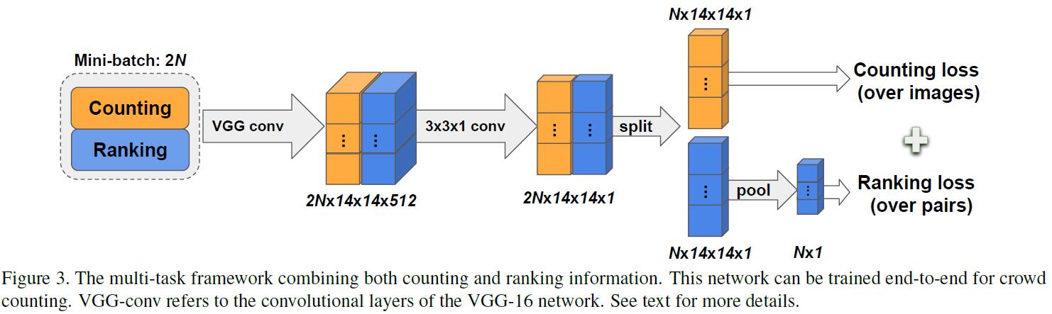

此外，为了进一步提高性能，作者采用了multi-scale sampling策略，即使用56——448 pixels之间varying size的square patches作为输入，作者发现这种multi-scale input可以显著提高模型性能。

Crowd ranking network

对于ranking network，我们将Euclidean loss替换为average pooling layer + ranking loss。首先，average pooling layer将density map转换为每个spatial unit $\hat{c}(I_i)$中person number的estimate。其中，
$$
\hat{c}(I_i)=\frac{1}{M}\sum_{j}\hat{y}_i (x_j)
$$

$x_j$ are the spatial coordinates of the density map, and $M = 14\times 14$ is the number of spatial units in the density map. The ranking which is on the total number of persons in the patch $\hat{C}_i$ also directly holds for its normalized version $\hat{c}_i$, since $\hat{C}(I_i)=M\times \hat{c}(I_i)$.

这里使用了pairwise ranking hinge loss：
$$
L_{r}=max(0, \hat{c}(I_2) - \hat{c}(I_1) + \epsilon)
$$
$\epsilon$是margin，但是在本文中设为0，我们假定 $\hat{c}(I_1)$ 的rank比 $\hat{c}(I_2)$ 高。

Ranking loss的梯度计算如下：
$$
\triangledown_{\theta}L_r=\begin{cases}
0 & \hat{c}(I_2) - \hat{c}(I_1) + \epsilon\leq 0\\
\triangledown_{\theta}\hat{c}(I_2) - \triangledown_{\theta}\hat{c}(I_1) & otherwise
\end{cases}
$$

When network outputs the correct ranking there is no backpropagated gradient. However, when the network estimates are not in accordance with the correct ranking the backpropagated gradient causes the network to increase its estimate for the patch with lower score and to decrease its estimate for the one with higher score (note that in backpropagation the gradient is subtracted).

在实现中，作者将图片作为one batch(for regression & ranking)更为有效，因此ranking loss可以被计算为：
$$
L_r=\sum_{i=1}^M \sum_{j\in S(i)}max(0, \hat{c}(I_j) - \hat{c}(I_i) + \epsilon)
$$

where $S(i)$ is the set of patches containing fewer people than patch $i$. Note that this relation is only defined for patches which are contained by patch $i$. In practice we sample minibatches of 25 images which contain 5 sets of 5 images which can be compared among them resulting in a total of $5\times (4 + 3 + 2 + 1) = 50$ pairs in one minibatch.

Combining counting and ranking data

Joint loss的叠加有以下3中方案：

• Ranking plus fine-tuning: In this approach the network is first trained on the large dataset of ranking data, and is next fine-tuned on the smaller dataset for which density maps are available.
• Alternating-task training: While ranking plus finetuning works well when the two tasks are closely related, it might perform bad for crowd counting because no supervision is performed to indicate what the network is actually supposed to count. Therefore, we propose to alternate between the tasks of counting and ranking. In practice we perform train for 300 minibatches on a single task before switching to the other, then repeat.
• Multi-task training: In the third approach, we add the self-supervised task as a proxy to the supervised counting task and train both simultaneously.
  $$
  L=L_c + \lambda L_r
  $$

Learning from Synthetic Data for Crowd Counting in the Wild

Paper: Learning from Synthetic Data for Crowd Counting in the Wild

这里介绍一篇CVPR’19上面一篇做counting的文章，主体思想比较简单，但是非常有意思 (利用GTA渲染的图片作为auxiliary data)。熟悉counting的同学都知道，给密集的图片标注是即容易出错、又难以标注的活。同时，玩过GTA游戏的同学也知道，现在最新版的GTA可以渲染出非常逼真的效果，那么可不可以利用GTA游戏渲染引起来手动生成synthetic data，然后再到target dataset上finetune呢？OK，现在问题是不是就转化成了如何去有效解决Transfer Learning中的domain adaptation问题了呢？

Pattern Recognition task中，feature matters! 因此之前很多counting领域的工作都是在设计discriminative的feature，或者设计更加优秀的DNN去学习更加discriminative的feature，常见的套路就是“multi-scale”、“context”、“hierarchical”等等，具体的可以参考上面的讲解，此处不再赘述。

为了有效解决transfer learning中的domain adaptation问题，作者提出了SSIM Embedding Cycle GAN来transfer synthetic scenes to realistic scenes。在训练过程中，作者使用了SSIM (Structural Similarity Index) Loss，它可以作为generator和original images中的penalty，使用了SSIM Loss的Cycle GAN能够得到比基础的Cycle GAN保留更多细节信息的图片。

注：SSIM is nothing new. 熟悉Image Quality Assessment的同学应该很熟悉。

Supervised Crowd Counting

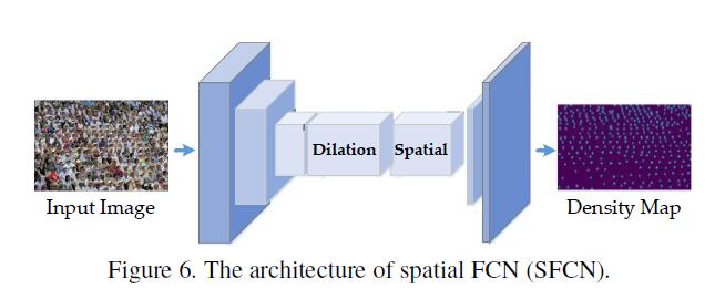
基础网络的设计方面，作者改进了著名的VGG16至FCN-VGG16模型，然后新增了一个Spatial Encoder与regression layer来回归counting点数量。网络结构SFCN结构如下图所示，其他的没啥好说的。

Crowd Counting via Domain Adaptation

接下来介绍一下本文的重点，即作者是如何使用SSIM Embedding Cycle GAN来将从GTA游戏中渲染的图片translate到photo-realistic images中的。

SSIM Embedding Cycle GAN

所谓Domain Adaptation，意思就是学习synthetic domain $\mathcal{S}$ 和real-world domain $\mathcal{R}$ 之间的某种translation mapping。其中，$\mathcal{S}$ 有图片 $I_{\mathcal{S}}$和count labels $L_{\mathcal{S}}$，而real-world domain $\mathcal{R}$ 只有图片 $I_\mathcal{R}$。因此，我们的任务就是给定图片 $I_{\mathcal{S}}$、count labels $L_{\mathcal{S}}$、图片 $I_\mathcal{R}$，来训练模型去预测 $\mathcal{R}$ 的density map。

不妨先来介绍一下Cycle GAN：
给定domain $\mathcal{S}$ 和domain $\mathcal{R}$，我们定义两个generator $G_{\mathcal{S}\to \mathcal{R}}$ 与 $G_{\mathcal{R}\to \mathcal{S}}$。在Cycle-consistent loss背景下，对于sample $i_{\mathcal{S}}$ 与 sample $i_{\mathcal{R}}$，我们的目标可以表示为：
$$
i_{\mathcal{S}}\to G_{\mathcal{S}\to \mathcal{R}}(i_{\mathcal{S}})\to G_{\mathcal{R}\to \mathcal{S}}(G_{\mathcal{S}\to \mathcal{R}}(i_{\mathcal{S}}))\approx i_{\mathcal{S}}
$$

同样地，对于 $i_{\mathcal{R}}$ 的优化目标，和上述 $i_{\mathcal{S}}$ 类似，只不过要将 $\mathcal{S}$ 和 $\mathcal{R}$ 进行逆转，此处不再赘述。

Cycle-consistent Loss定义为Cycle Architecture上的$L_1$ penalty：
$$
\mathcal{L}_{cycle}(G_{\mathcal{S}\to \mathcal{R}}, G_{\mathcal{R}\to \mathcal{S}}, \mathcal{S}, \mathcal{R})=
$$
$$
\mathbb{E}_{i_{\mathcal{S}}\sim I_{\mathcal{S}}}[|G_{\mathcal{R}\to \mathcal{S}}(G_{\mathcal{S}\to \mathcal{R}}(i_{\mathcal{S}})) - i_{\mathcal{S}}|_1] +
$$
$$
\mathbb{E}_{i_{\mathcal{R}}\sim I_{\mathcal{R}}}[|G_{\mathcal{S}\to \mathcal{R}}(G_{\mathcal{R}\to \mathcal{S}}(i_{\mathcal{R}})) - i_{\mathcal{R}}|_1]
$$

然后，discriminator $D_{\mathcal{R}}$ 被用来判别images是 $I_{\mathcal{R}}$ 还是 $G_{\mathcal{S}\to \mathcal{R}}(I_{\mathcal{S}})$，$D_{\mathcal{S}}$ 被用来判别images是 $I_{\mathcal{S}}$ 还是 $G_{\mathcal{R}\to \mathcal{S}}(I_{\mathcal{R}})$。

因此，training的adverserial loss为：
$$
\mathcal{L}_{GAN}(G_{\mathcal{S}\to \mathcal{R}}, D_{\mathcal{R}}, \mathcal{S}, \mathcal{R})=
\mathbb{E}_{i_{\mathcal{R}}\sim I_{\mathcal{R}}}[log(D_{\mathcal{R}}(i_{\mathcal{R}}))]+
\mathbb{E}_{i_{\mathcal{S}}\sim I_{\mathcal{S}}}[log(D_{\mathcal{S}}(i_{\mathcal{S}}))]
$$

因此，总体的Loss Function定义为：
$$
\mathcal{L}_{CycleGAN}(G_{\mathcal{S}\to \mathcal{R}},G_{\mathcal{R}\to \mathcal{S}},D_{\mathcal{R}}, D_{\mathcal{S}}, \mathcal{S}, \mathcal{R})=
$$
$$
\mathcal{L}_{GAN}(G_{\mathcal{S}\to \mathcal{R}}, D_{\mathcal{R}}, \mathcal{S}, \mathcal{R})+
$$
$$
\mathcal{L}_{GAN}(G_{\mathcal{R}\to \mathcal{S}}, D_{\mathcal{S}}, \mathcal{S}, \mathcal{R})+
$$
$$
\lambda \mathcal{L}_{cycle}(G_{\mathcal{R}\to \mathcal{S}}, G_{\mathcal{S}\to \mathcal{R}}, \mathcal{S}, \mathcal{R})
$$

下面介绍一下本文另一个重点——SSIM Embedding Cycle-consistent Loss，在crowd场景下，high-density和low-density最大的区别就是local pattern和texture features。然而，若直接使用原始的Cycle-consistent loss会丢失掉很多细节信息，因此作者借用了Image Quality Assessment领域中经常使用的SSMI ($SSIM\in [-1, 1]$，若SSIM越大，则说明该图片质量越高)。SSIM Embedding能够保证original images和reconstructed images有较高的结构相似性(Structural Similarity)，因此可促进两个generator在training过程中保持一定程度的SS。

SE Cycle-GAN的目标如下：
$$
\mathcal{L}_{SE_{cycle}}(G_{\mathcal{S}\to \mathcal{R}},G_{\mathcal{R}\to \mathcal{S}},\mathcal{S},\mathcal{R})=
$$
$$
\mathbb{E}_{i_{\mathcal{S}}\sim I_{\mathcal{S}}}[1-SSIM(i_{\mathcal{S}},G_{\mathcal{R}\to \mathcal{S}}(G_{\mathcal{S}\to \mathcal{R}}(i_{\mathcal{S}})))]+
$$
$$
\mathbb{E}_{i_{\mathcal{R}}\sim I_{\mathcal{R}}}[1-SSIM(i_{\mathcal{R}},G_{\mathcal{S}\to \mathcal{R}}(G_{\mathcal{R}\to \mathcal{S}}(i_{\mathcal{R}})))]
$$

最终的Loss如下：
$$
\mathcal{L}_{ours}(G_{\mathcal{S}\to \mathcal{R}},G_{\mathcal{R}\to \mathcal{S}},D_{\mathcal{R}}, D_{\mathcal{S}}, \mathcal{S}, \mathcal{R})=
$$
$$
\mathcal{L}_{GAN}(G_{\mathcal{S}\to \mathcal{R}}, D_{\mathcal{R}}, \mathcal{S}, \mathcal{R})+
$$
$$
\mathcal{L}_{GAN}(G_{\mathcal{R}\to \mathcal{S}}, D_{\mathcal{S}}, \mathcal{S}, \mathcal{R})+
$$
$$
\lambda \mathcal{L}_{cycle}(G_{\mathcal{R}\to \mathcal{S}}, G_{\mathcal{S}\to \mathcal{R}}, \mathcal{S}, \mathcal{R})+
$$
$$
\mu \mathcal{L}_{SE_{cycle}}(G_{\mathcal{S}\to \mathcal{R}},G_{\mathcal{R}\to \mathcal{S}},\mathcal{S},\mathcal{R})
$$

Leveraging Heterogeneous Auxiliary Tasks to Assist Crowd Counting

Paper: Leveraging Heterogeneous Auxiliary Tasks to Assist Crowd Counting

Basic Ideas

Leveraging Heterogeneous Auxiliary Tasks to Assist Crowd Counting是发表在CVPR’19上的成果，main idea也非常简单，顾名思义，即用multi-task learning的方法来regularize模型，从而提高main task的performance，之前有做过Face Analysis的Multi-task Learning，所以这篇大体上自然非常熟悉了。

说到Counting，其本质上可视为一个Regression问题，严格意义上讲叫作density map regression，所以和其他machine learning task一样，feature matters! 不少research work专注于设计或融合multi-scale, context-aware features来产生更加robust的features。这篇文章主要是通过MTL的方法来向网络中embed semantic/geometric/numeric的信息，从而获取更加discriminative and robust的features来提高performance。

• 对于geometric attribute，作者使用monocular depth prediction来强调relative depth variantions。
• 对于semantic attribute，作者使用crowd segmentation来highlight foreground。
• 对于numeric attribute，作者直接回归count estimation。

虽然引入了多个任务，但是这些auxiliary task却并不需要额外的human-annotation，因为上述3个auxiliary task所需要的annotation均可以通过现有pre-trained model生成，或直接通过其他方式计算得来。

Learning of the auxiliary tasks will drive the intermediate features of the backbone CNN to embed desired information on geometry, semantics and the overall density level, which benefits the generation of robust features against the scale variations and clutter background.

AT-CNN的网络结构如下图所示：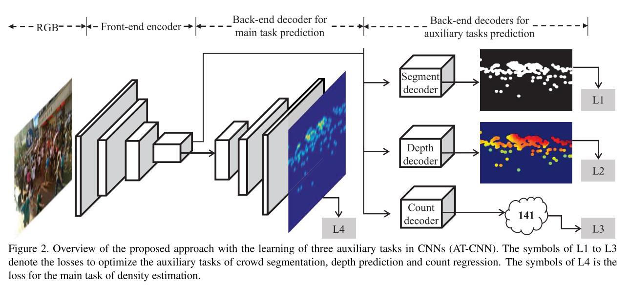

Methodology

Auxiliary Tasks Prediction Based

• Attentive Crowd Segmentation
  由于crowd scene occlusion和clutter background现象非常严重，crowd density通常noisy。为了解决该问题，作者引入了segmentation task来purify output prediction。

  Ground-truth labels for crowd segmentation can be in- ferred from the dotted annotations of pedestrians provided in counting dataset [36, 35] by simple binarization as shown in Figure 3.

  令$X$代表input crowd image，$S$代表gt attentive crowd segmentation map，Segmentation decoder的loss如下：
  $$
  L_1=\frac{1}{|X|}\sum_{(i,j)\in X}t_{ij}log o_{ij} + (1-t_{ij})log(1 - o_{ij})
  $$
  其中，$t_{ij}\in \{0,1\}$为1时代表foreground，为0代表background，$o_{ij}$代表pixel-wise probability。

• Distilled Depth Prediction
  该task的引入主要是为了处理perspective distortion现象。
  In the regions with larger depth values, the objects have smaller sizes and should be adversely assigned with larger density values to guarantee their summation gives accurate counts. By inferring the depth maps, the front-end CNN is imposed to take care of the scene geometry and hence gains the awareness of the intra-image scale variations, which will help generate more discriminative features for scale-aware density estimation.

  在这里作者使用pre-trained DCNF来预测single-image depth，由于DCNF并不能完美adapt to crowd counting task中，因此作者计算了distilled depth map $D$，distilled depth map仅仅保留了attentive target areas的depth information。其计算方式如下：
  $$
  D=S\bigodot D_{raw}
  $$
  $\bigodot$代表Hadamard matrix multiplication. With the distilled depth as the supervision for depth prediction, the front-end CNN is desired to be especially aware of the depth relationships/scale variation between those attentive areas with target objects.

  Depth map prediction的Loss如下：
  $$
  L_2=\frac{1}{|D|}\sum_{(i,j)\in D}|\hat{D}_{ij}-D_{ij}|_2^2
  $$

• Crowd Count Regression
  从feature map直接regress到count number，MSE Loss作为supervision。

Main Tasks Prediction

在文中，作者对每个dotted annotations使用2D Gaussian Kernels来生成density map，main task的decoder在density map $\hat{Y}$上采用$L_2$ loss:
$$
L_4 = \frac{1}{|Y|}\sum_{(i,j)\in Y}|\hat{Y}_{ij} - Y_{ij}|_2^2
$$

既然是MTL，那么overall optimization当然就是各个loss的linear combination啦:
$$
L_{mt}=\sum_{i=1}^4 \lambda_i L_i
$$

接下来就是实验了，当然是碾压各种prior arts。此外，作者还分析了不同weights $\lambda$对performance的影响：

Too small weights are hard to contribute to the main tasks while too large weights will drift the feature representations and deteriorate the performances. Similar situations can be be observed for the crowd segmentation loss and the count regression loss.

Reference

1. Zhang, Yingying, et al. “Single-image crowd counting via multi-column convolutional neural network.” Proceedings of the IEEE conference on computer vision and pattern recognition. 2016.
2. Shen, Zan, et al. “Crowd Counting via Adversarial Cross-Scale Consistency Pursuit.” Proceedings of the IEEE Conference on Computer Vision and Pattern Recognition. 2018.
3. Liu, Xialei, Joost van de Weijer, and Andrew D. Bagdanov. “Leveraging Unlabeled Data for Crowd Counting by Learning to Rank.” Proceedings of the IEEE Conference on Computer Vision and Pattern Recognition. 2018.
4. Marsden, Mark, et al. “People, Penguins and Petri Dishes: Adapting Object Counting Models To New Visual Domains And Object Types Without Forgetting.” Proceedings of the IEEE Conference on Computer Vision and Pattern Recognition. 2018.
5. Liu, Jiang, et al. “Decidenet: Counting varying density crowds through attention guided detection and density estimation.” Proceedings of the IEEE Conference on Computer Vision and Pattern Recognition. 2018.
6. Hinami, Ryota, Tao Mei, and Shin’ichi Satoh. “Joint detection and recounting of abnormal events by learning deep generic knowledge.” Proceedings of the IEEE International Conference on Computer Vision. 2017.
7. Hsieh, Meng-Ru, Yen-Liang Lin, and Winston H. Hsu. “Drone-based object counting by spatially regularized regional proposal network.” The IEEE International Conference on Computer Vision (ICCV). Vol. 1. 2017.
8. Sam, Deepak Babu, Shiv Surya, and R. Venkatesh Babu. “Switching convolutional neural network for crowd counting.” Proceedings of the IEEE Conference on Computer Vision and Pattern Recognition. Vol. 1. No. 3. 2017.
9. Chattopadhyay, Prithvijit, et al. “Counting everyday objects in everyday scenes.” Proceedings of the IEEE Conference on Computer Vision and Pattern Recognition. 2017.
10. Ranjan, Viresh, Hieu Le, and Minh Hoai. “Iterative crowd counting.” Proceedings of the European Conference on Computer Vision (ECCV). 2018.
11. Cao, Xinkun, et al. “Scale aggregation network for accurate and efficient crowd counting.” Proceedings of the European Conference on Computer Vision (ECCV). 2018.
12. Wang, Qi, et al. “Learning from Synthetic Data for Crowd Counting in the Wild.” Proceedings of the IEEE Conference on Computer Vision and Pattern Recognition. (2019).
13. Zhao, Muming, et al. “Leveraging Heterogeneous Auxiliary Tasks to Assist Crowd Counting.” Proceedings of the IEEE Conference on Computer Vision and Pattern Recognition. 2019.