
Introduction
人脸识别(Face Recognition)是工业界和学术界都非常火热的一个方向,并且已经催生出许多成功的应用落地场景,比如刷脸支付、安检等。而Face Recognition最大的突破也是由Deep Learning Architecture + 一系列精巧的Loss Function带来的。本文旨在对Face Recognition领域里的一些经典Paper进行梳理,详情请参阅Reference部分的Paper原文。
@LucasXU注:本文长期更新。
Face Recognition as N-Categories Classification Problems
在Metric Learning里的一系列优秀的Loss还未被引入Face Recognition之前,Face Verification/Identification一个非常直观的想法就是直接train 一个 n-categories classifier。然后将最后一层的输出作为input image的特征,再选取合适的distance metric来决定这两张脸是否属于同一个人。这种做法的一些经典工作就是DeepID。这篇Paper发表在CVPR2014上面,属于非常古董的模型了,鉴于近年来已经几乎不这么做了,所以本文仅仅象征性地回顾一下这几篇具有代表性的Paper。我们会把讨论重心放在Metric Learning的一系列Loss上。
Paper: Deep learning face representation from predicting 10,000 classes
这篇Paper其实idea非常简单,就是把Face Recognition问题转换为一个$N$-类Classification问题,其中$N$代表dataset中identity的数量。为了增强feature representation能力,作者也将各个facial region的特征做concatenation。DeepID的Architecture如下: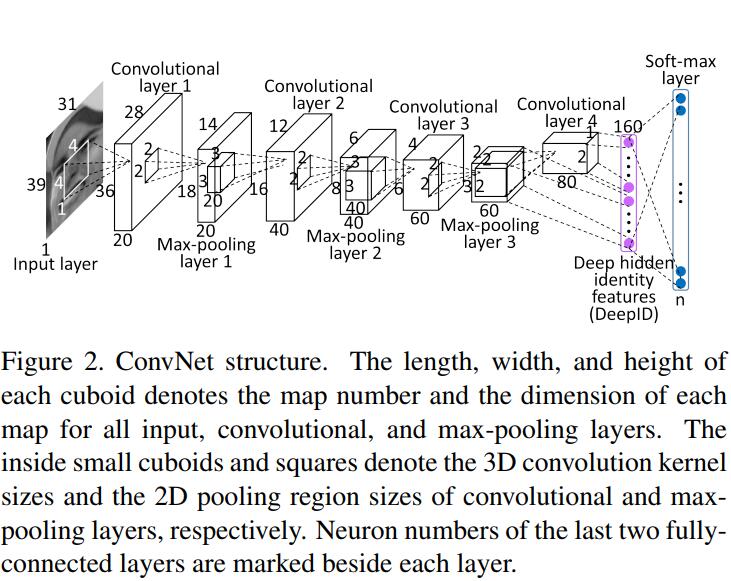
注意到DeepID的输入部分,除了后一个conv layer的feature map之外,还有前一个max-pooling的输出,这样做的好处在于Network能够获取multi-scale的input,也可以视为一种skipping layer(将lower level feature和higher level feature做feature fusion)。那么最后一个hidden layer的输入就是这样子的:
$$
y_j=max(0, \sum_i x_i^1\cdot w_{i,j}^1 + \sum_i x_i^2\cdot w_{i,j}^2 + b_j)
$$
另外,作者在实验中意识到,随着identity 数量的增加,整个网络的feature representation learning和performance都会随之增加。DeepID在LFW上达到了97.45%的精度。
FaceNet
Google的FaceNet是我个人认为在Face Recognition领域里一篇非常insightful的Paper,通过引入triplets并直接在Euclidean Space作为feature vector度量,FaceNet在LFW上达到了99.63%的效果。
Paper: Facenet: A unified embedding for face recognition and clustering.
What is FaceNet?
FaceNet的Idea其实也比较简单。简而言之呢,就是通过DNN学习一种Euclidean Embedding,来使得inter-class更加compact,inter-class更加地separable,这就是本文的核心角色——Triplet Loss。
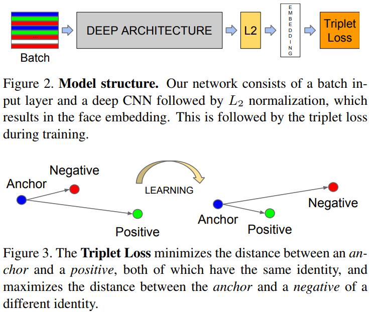
Details of Triplet Loss
Triplet Embedding是通过一个Network将输入$x$映射到$d$-维输出$f(x)\in \mathbb{R}^d$,文章中将其做了一个Normalization,即$||f(x)||_2=1$。Triplet Loss的目的就是为了找到一个person的anchor $x_i^a$,使得它与相同identity的positive images $x_i^p$更加地close,而与不同identity的negative images更加地separate。写成公式就是:
$$
||x_i^a-x_i^p||_2^2 + \alpha < ||x_i^a-x_i^n||_2^2 \quad \forall (x_i^a,x_i^p,x_i^n)\in \mathcal{T}
$$
$\alpha$就代表margin,那么Minimization of Triplet Loss就是:
$$
\sum_{i}^N [||f(x_i^a)-f(x_i^p)||_2^2 - ||f(x_i^a)-f(x_i^n)||_2^2 + \alpha ]_+
$$
Triplet Loss确定了,那么下一步就是如何选择合适的Triplets。
Triplet Selection
为了保证快速收敛,我们需要violate triplet的constraint,即挑选anchor $x_i^a$,来挑选hard positive $x_i^p$来满足$\mathop{argmax} \limits_{x_i^p}||f(x_i^a)-f(x_i^p)||_2^2$,以及hard negative $x_i^n$来满足$\mathop{argmin} \limits_{x_i^p}||f(x_i^a)-f(x_i^n)||_2^2$。
@LucasXU注:读者仔细体会一下这里和triplet loss definition的区别,为啥是相反的?这里可视为一种hard negative mining。
在整个training set上计算$argmax$和$argmin$是不太现实的,文中采取了两个做法:
- 训练每$n$步离线来生成triplets,使用most recent network checkpoint和dataset的子集来计算$argmax$和$argmin$。
- 在线生成triplets,这种做法可视为在一个mini-batch选择hard positive/negative exemplars。
Selecting the hardest negatives can in practice lead to bad local minima early on in training,specifically it can result in a collapsed model (i.e. $f(x) = 0$). In order to mitigate this, it helps to select $x^n_i$ such that:
$$
||f(x_i^a)-f(x_i^p)||_2^2 < ||f(x_i^a)-f(x_i^n)||_2^2
$$
We call these negative exemplars semi-hard, as they are further away from the anchor than the positive exemplar, but still hard because the squared distance is close to the anchorpositive distance. Those negatives lie inside the margin $\alpha$.
Experiments
对于Face Verification Task,判断两张图是否为一个人,我们仅需比较这两个特征向量的squared $L_2$ distance $D(x_i,x_j)$是否超过了某个阈值即可。
- True Accepts代表face pairs $(i,j)被正确分类到同一个identity$:
$TA(d)=\{(i,j)\in \mathcal{P}_{same},\quad with \quad D(x_i,x_j)\leq d\}$ - False Accepts代表face pairs $(i,j)被错误分类到同一个identity$:
$FA(d)=\{(i,j)\in \mathcal{P}_{diff},\quad with \quad D(x_i,x_j)\leq d\}$
Center Loss
Paper: A discriminative feature learning approach for deep face recognition
Face Recognition领域,除了设计更加优秀的Network Architecture,也有另一个方向的工作是在设计更加优秀的Loss。Center Loss就是其中之一。和FaceNet中使用Triplet Loss的目的一样,Center Loss依然是为了使得intra-class more compact and inter-class more separate。本文就来简要介绍一下Center Loss。
Center Loss通过学习每一个类的中心向量,来同时更新这个center,以及最小化deep features和其对应class的centers之间的距离。CNN的Loss为Softmax Loss与Center Loss的加权。Softmax Loss仅仅会让不同的class分开,但Center Loss还会使得相同class的deep features更加靠近类的centers。通过这种joint supervision(Softmax + Center Loss),不仅仅inter-class的difference被加大了,而且intra-class的variantions也被减小了。因此便可以学得更加discriminative的feature representation。这便是Center Loss的大致idea。
What is Center Loss?
Softmax Loss是这样的:
$$
\mathcal{L}_S=-\sum_{i=1}^m log\frac{e^{W_{y_i}^Tx_i+b_{y_i}}}{\sum_{j=1}^n e^{W_j^Tx_i+b_j}}
$$
Center Loss则是这样的:
$$
\mathcal{L}_C=\frac{1}{2}\sum_{i=1}^m ||x_i-c_{y_i}||_2^2
$$
为了更新center vector $c_{y_i}$,文中采取的做法是在每一个mini-batch中进行更新(而不是在整个training set中更新),然后center vector $c_{y_i}$的计算为相关class feature的平均值。此外,为了避免mislabeled samples,我们使用$\alpha$来控制center vector的learning rate。Center Loss的梯度求导可以表示为:
$$
\frac{\partial \mathcal{L}_C}{\partial x_i}=x_i - c_{y_i}
$$
$$
\Delta c_j=\frac{\sum_{i=1}^m \delta(y_i=j)\cdot (c_j-x_i)}{1+\sum_{i=1}^m\delta(y_i=j)}
$$
where $\delta(condition) = 1$ if the condition is satisfied, and $\delta(condition) = 0$ if not. $\alpha$ is restricted in $[0, 1]$. We adopt the joint supervision of softmax loss and center loss to train the CNNs for discriminative feature learning. The formulation is given in Eq. 5.
$$
\mathcal{L}=\mathcal{L}_S+\lambda \mathcal{L}_C=-\sum_{i=1}^m log\frac{e^{W_{y_i}^Tx_i + b_{y_i}}}{\sum_{j=1}^n e^{W_j^Tx_i + b_j}} + \frac{\lambda}{2} \sum_{i=1}^m ||x_i-c_{y_i}||_2^2
$$
整个学习算法如下: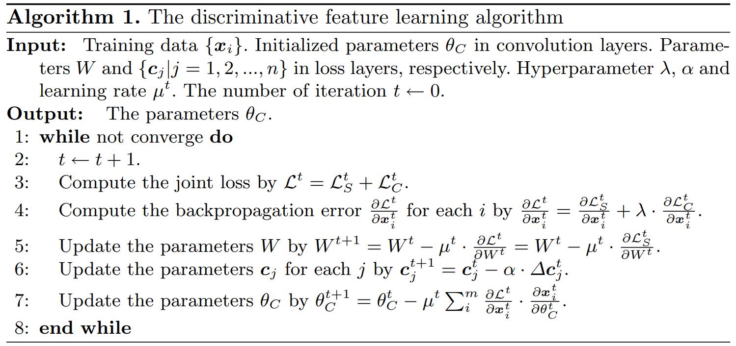
网络结构如下: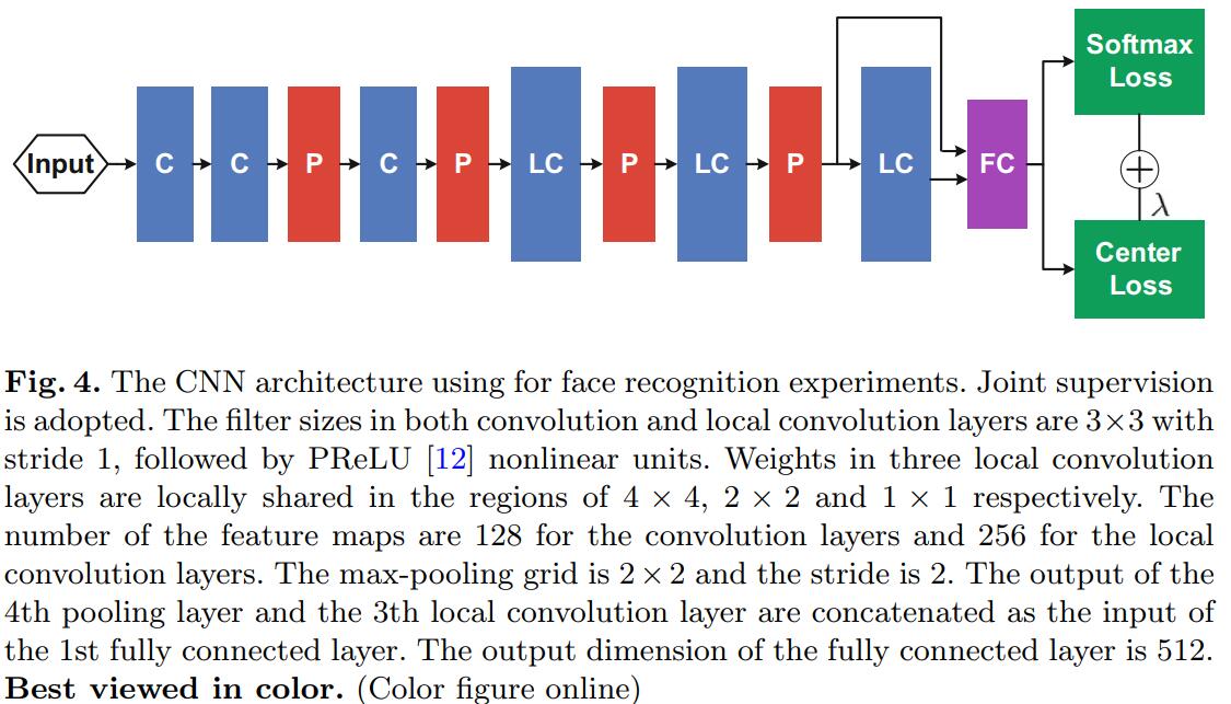
Center Loss的好处在于:
- Joint supervision of Softmax Loss and Center Loss能够大大加强DCNN的feature learning能力。
- 其他Metric Learning的Loss例如Triplet Loss, Contractive Loss等pairs selection是非常麻烦的一件事情,但是Center Loss则不需要复杂的triplet pairs selection。
网络学习完成,在做Face Verification/Identification时,第一个 FC Layers的feature被当作特征,同时,我们也将水平翻转图片的feature进行concatenation,作为最终的face feature,PCA降维之后,Cosine Distance, Nearest Neighbor and Threshold comparison用来作为判断是否为同一个人的依据。
SphereFace
Paper: Sphereface: Deep hypersphere embedding for face recognition
SphereFace是发表在CVPR2017上的Paper,也是Face Recognition领域里一篇非常insightful的Paper。自从FaceNet起,近些年来人脸识别领域大多都是在做相同的事情:
设计更加优秀的Loss,来使得intra-class更加compact,inter-class更加separable,从而提升识别精度。SphereFace自然也不例外。
SphereFace里提出的Loss叫作A-Softmax(Angular-Softmax),来让DCNN学习angularly discriminative features。A-Softmax可以看作是在hyper-sphere施加了discriminative constraints,来满足faces分布在相同流形的先验。此外,A-Softmax也是基于margin的,angular margin可以通过参数m进行调节。m越大会得到更大的angular margin(即流形上更discriminative的feature distribution)。
根据testing protocol,人脸识别可以分为以下两类:
- Close-set protocol: For closed-set protocol, all testing identities are predefined in training set. It is natural to classify testing face images to the given identities. In this scenario, face verification is equivalent to performing identification for a pair of faces respectively (see left side of Fig. 1). Therefore, closed-set FR can be well addressed as a classification problem, where features are expected to be separable.
- Open-set protocol: For open-set protocol, the testing identities are usually disjoint from the training set, which makes FR more challenging yet close to practice. Since it is impossible to classify faces to known identities in training set, we need to map faces to a discriminative feature space. In this scenario, face identification can be viewed as performing face verification between the probe face and every identity in the gallery (see right side of Fig. 1). Open-set FR is essentially a metric learning problem, where the key is to learn discriminative large-margin features.
良好的facial representation需要满足这样的条件:maximal intra-class distance需要比minimal inter-class distance还要小。一些比较老的深度学习算法将人脸识别视为一个N-category classification问题,但是Softmax Loss学习的feature不够discriminative。为了解决这个问题,后来一大批工作都是在设计更加优秀的Loss Function(例如Triplet Loss, Center Loss, Contrastive Loss等等)。但是Center Loss仅仅显示地促使intra-class更加compact,Contractive Loss和Triplet Loss都不能对每个sample都施加constrain,因此需要carefully designed pairs mining。
之前的工作都是在Euclidean Space上施加的constraint,但这样未必是有效的。
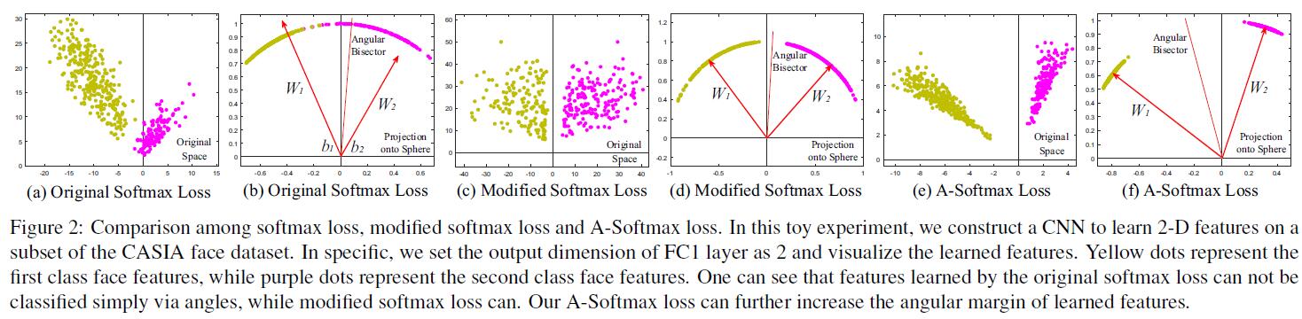
It seems to be a widely recognized choice to impose Euclidean margin to learned features, but a question arises: Is Euclidean margin always suitable for learning discriminative face features? To answer this question, we first look into how Euclidean margin based losses are applied to FR. Most recent approaches [25, 28, 34] combine Euclidean margin based losses with softmax loss to construct a joint supervision. However, as can be observed from Fig. 2, the features learned by softmax loss have intrinsic angular distribution (also verified by [34]). In some sense, Euclidean margin based losses are incompatible with softmax loss, so it is not well motivated to combine these two type of losses.
而在SphereFace中,作者选用了Angular Margin来代替Euclidean Margin。
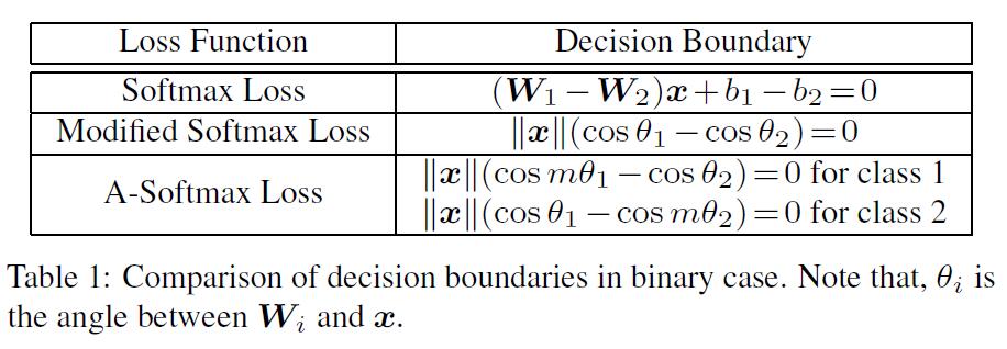
In this paper, we propose to incorporate angular margin instead. We start with a binary-class case to analyze the softmax loss. The decision boundary in softmax loss is $(W_1−W_2)x+b_1−b_2=0$, where $W_i$ and $b_i$ are weights and bias in softmax loss, respectively. If we define $x$ as a feature vector and constrain $||W_1||=||W_2||=1$ and $b_1=b_2=0$, the decision boundary becomes $||x||(cos(\theta_1)− cos(\theta_2))=0$, where $\theta_i$ is the angle between $W_i$ and $x$. The new decision boundary only depends on $\theta_1$ and $\theta_2$. Modified softmax loss is able to directly optimize angles, enabling CNNs to learn angularly distributed features (Fig. 2).
Compared to original softmax loss, the features learned by modified softmax loss are angularly distributed, but not necessarily more discriminative. To the end, we generalize the modified softmax loss to angular softmax (A-Softmax) loss. Specifically, we introduce an integer $m (m\geq 1)$ to quantitatively control the decision boundary. In binaryclass case, the decision boundaries for class 1 and class 2 become $||x||(cos(m\theta_1)−cos(\theta_2))=0$ and $||x||(cos(\theta_1)− cos(m\theta_2))=0$, respectively. $m$ quantitatively controls the size of angular margin. Furthermore, A-Softmax loss can be easily generalized to multiple classes, similar to softmax loss. By optimizing A-Softmax loss, the decision regions become more separated, simultaneously enlarging the inter-class margin and compressing the intra-class angular distribution.
A-Softmax loss has clear geometric interpretation. Supervised by A-Softmax loss, the learned features construct a discriminative angular distance metric that is equivalent to geodesic distance on a hypersphere manifold. A-Softmax loss can be interpreted as constraining learned features to be discriminative on a hypersphere manifold, which intrinsically matches the prior that face images lie on a manifold [14, 5, 31]. The close connection between A-Softmax loss and hypersphere manifolds makes the learned features more effective for face recognition. For this reason, we term the learned features as SphereFace.
Moreover, A-Softmax loss can quantitatively adjust the angular margin via a parameter $m$, enabling us to do quantitative analysis. In the light of this, we derive lower bounds for the parameter m to approximate the desired open-set FR criterion that the maximal intra-class distance should be smaller than the minimal inter-class distance.
Preliminary
Metric Learning
提到Face Recognition,就不得不提Metric Learning了,那么究竟什么是Metric Learning呢?
Metric learning aims to learn a similarity (distance) function. Traditional metric learning [36, 33, 12, 38] usually learns a matrix A for a distance metric $||x_1-x_2||_A=\sqrt{(x_1-x_2)^TA(x_1-x_2)}$ upon the given features $x_1$, $x_2$. Recently, prevailing deep metric learning [7, 17, 24, 30, 25, 22, 34] usually uses neural networks to automatically learn discriminative features $x_1, x_2$ followed by a simple distance metric such as Euclidean distance $||x_1-x_2||_2$. Most widely used loss functions for deep metric learning are contrastive loss [1, 3] and triplet loss [32, 22, 6], and both impose Euclidean margin to features.
L-Softmax loss [16] also implicitly involves the concept of angles. As a regularization method, it shows great improvement on closed-set classification problems. Differently, A-Softmax loss is developed to learn discriminative face embedding. The explicit connections to hypersphere manifold makes our learned features particularly suitable for open-set FR problem, as verified by our experiments. In addition, the angular margin in A-Softmax loss is explicitly imposed and can be quantitatively controlled (e.g. lower bounds to approximate desired feature criterion), while [16] can only be analyzed qualitatively.
Deep Hypersphere Embedding
Introducing Angular Margin to Softmax Loss
Assume a learned feature $x$ from class 1 is given and $\theta_i$ is the angle between $x$ and $W_i$, it is known that the modified softmax loss requires $cos(\theta_1)>cos(\theta_2)$ to correctly classify $x$. But what if we instead require $cos(m\theta_1)>cos(\theta_2)$ where $m\geq 2$ is a integer in order to correctly classify $x$? It is essentially making the decision more stringent than previous, because we require a lower bound of $cos(\theta_1)$ to be larger than $cos(\theta_2)$. The decision boundary for class 1 is $cos(m\theta_1)= cos(\theta_2)$. Similarly, if we require $cos(m\theta_2)>cos(\theta_1)$ to correctly classify features from class 2, the decision boundary for class 2 is $cos(m\theta_2)=cos(\theta_1)$. Suppose all training samples are correctly classified, such decision boundaries will produce an angular margin of $\frac{m-1}{m+1}\theta_2^1$ where $\theta_2^1$ is the angle between $W_1$ and $W_2$. From angular perspective, correctly classifying $x$ from identity 1 requires $\theta_1<\frac{\theta_2}{m}$, while correctly classifying $x$ from identity 2 requires $\theta_2<\frac{\theta_1}{m}$. Both are more difficult than original $\theta_1<\theta_2$ and $\theta_2<\theta_1$, respectively. By directly formulating this idea into the modified softmax loss Eq. (5), we have:
$$
L_{ang}=\frac{1}{N}\sum_{i}-log(\frac{e^{|x_i|cos(m\theta_{y_i,i})}}{e^{|x_i|cos(m\theta_{y_i,i})} + \sum_{j\neq y_i}e^{|x_i|cos(m\theta_{j,i})}})
$$
where $\theta_{y_i,i}$ has to be in the range of $[0, \frac{\pi}{m}]$. In order to get rid of this restriction and make it optimizable in CNNs, we expand the definition range of $cos(\theta_{y_i,i})$ by generalizing it to a monotonically decreasing angle function $\psi(\theta_{yi,i})$ which should be equal to $cos(\theta_{y_i,i})$ in $[0, \frac{\pi}{m}]$. Therefore our proposed A-Softmax loss is formulated as:
$$
L_{ang}=\frac{1}{N}\sum_{i}-log(\frac{e^{|x_i|\psi(\theta_{y_i,i})}}{e^{|x_i|\psi(\theta_{y_i,i})} + \sum_{j\neq y_i}e^{|x_i|cos(\theta_{j,i})}})
$$
in which we define $\psi(\theta_{y_i,i})=(-1)^kcos(m\theta_{y_i,i})-2k, \theta_{y_i,i}\in [\frac{k\pi}{m},\frac{(k+1)\pi}{m}]$ and $k\in [0, m-1]$. $m\geq 1$ is an integer that controls the size of angular margin. When $m=1$, it becomes the modified softmax loss.
The justification of A-Softmax loss can also be made from decision boundary perspective. A-Softmax loss adopts different decision boundary for different class (each boundary is more stringent than the original), thus producing angular margin. The comparison of decision boundaries is given in Table 1. From original softmax loss to modified softmax loss, it is from optimizing inner product to optimizing angles. From modified softmax loss to A-Softmax loss, it makes the decision boundary more stringent and separated. The angular margin increases with larger m and be zero if $m=1$.
Supervised by A-Softmax loss, CNNs learn face features with geometrically interpretable angular margin. Because ASoftmax loss requires $W_i=1, b_i=0$, it makes the prediction only depends on angles between the sample $x$ and $W_i$. So $x$ can be classified to the identity with smallest angle. The parameter $m$ is added for the purpose of learning an angular margin between different identities.
Hypersphere Interpretation of A-Softmax Loss
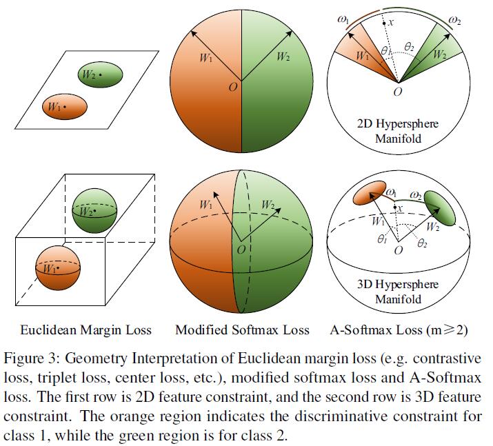
A-Softmax loss is equivalent to learning features that are discriminative on a hypersphere manifold, while Euclidean margin losses learn features in Euclidean space.
To simplify, We take the binary case to analyze the hypersphere interpretation. Considering a sample $x$ from class 1 and two column weights $W_1,W_2$, the classification rule for A-Softmax loss is $cos(m\theta_1)>cos(\theta_2)$, equivalently $m\theta_1< \theta_2$. Notice that $\theta_1, \theta_2$ are equal to their corresponding arc length $\omega_1,\omega_2$ on unit hypershere $\{v_j,\forall j| \sum_j v_j^2=1,v\geq 0\}$. Because $|W|_1=|W|_2=1$, the decision replies on the arc length $\omega_1$ and $\omega_2$. The decision boundary is equivalent to $m\omega_1=\omega_2$, and the constrained region for correctly classifying $x$ to class 1 is $m\omega_1<\omega_2$. Geometrically speaking, this is a hypercircle-like region lying on a hypersphere manifold.
Note that larger $m$ leads to smaller hypercircle-like region for each class, which is an explicit discriminative constraint on a manifold. For better understanding, Fig. 3 provides 2D and 3D visualizations. One can see that A-Softmax loss imposes arc length constraint on a unit circle in 2D case and circle-like region constraint on a unit sphere in 3D case. Our analysis shows that optimizing angles with A-Softmax loss essentially makes the learned features more discriminative on a hypersphere.
Discussions About A-Softmax Loss
Why angular margin. First and most importantly, angular margin directly links to discriminativeness on a manifold, which intrinsically matches the prior that faces also lie on a manifold. Second, incorporating angular margin to softmax loss is actually a more natural choice. As Fig. 2 shows, features learned by the original softmax loss have an intrinsic angular distribution. So directly combining Euclidean margin constraints with softmax loss is not reasonable.
Comparison with existing losses. In deep FR task, the most popular and well-performing loss functions include contrastive loss, triplet loss and center loss. First, they only impose Euclidean margin to the learned features (w/o normalization), while ours instead directly considers angular margin which is naturally motivated. Second, both contrastive loss and triplet loss suffer from data expansion when constituting the pairs/triplets from the training set, while ours requires no sample mining and imposes discriminative constraints to the entire mini-batches (compared to contrastive and triplet loss that only affect a few representative pairs/triplets).
Reference
- Sun, Yi, Xiaogang Wang, and Xiaoou Tang. “Deep learning face representation from predicting 10,000 classes.” Proceedings of the IEEE conference on computer vision and pattern recognition. 2014.
- Schroff, Florian, Dmitry Kalenichenko, and James Philbin. “Facenet: A unified embedding for face recognition and clustering.” Proceedings of the IEEE conference on computer vision and pattern recognition. 2015.
- Wen Y, Zhang K, Li Z, Qiao Y. A discriminative feature learning approach for deep face recognition. In European Conference on Computer Vision 2016 Oct 8 (pp. 499-515). Springer, Cham.
- Wang F, Xiang X, Cheng J, Yuille AL. Normface: L2 hypersphere embedding for face verification. InProceedings of the 2017 ACM on Multimedia Conference 2017 Oct 23 (pp. 1041-1049). ACM.
- Liu, Weiyang, et al. “Sphereface: Deep hypersphere embedding for face recognition.” The IEEE Conference on Computer Vision and Pattern Recognition (CVPR). Vol. 1. 2017.
- Hadsell, Raia, Sumit Chopra, and Yann LeCun. “Dimensionality reduction by learning an invariant mapping.” null. IEEE, 2006.