Introduction
RNN(Recurrent Neural Network)是一类专门处理序列数据的网络。RNN主要在NLP领域有着非常广泛的应用,也是当今火热的Deep Learning的其中模型之一。RNN在模型的不同部分共享参数,从而使得模型能够扩展到不同形式的样本并进行泛化。
展开Computational Graph
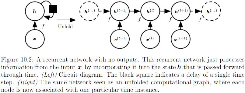
我们可以用一个函数$g^{(t)}$代表经过 $t$ 步展开后的循环:
$$
h^{(t)}=g^{(t)}(x^{(t)}, x^{(t-1)}, x^{(t-2)}, \cdots, x^{(1)})=f(h^{(t-1)}, x^{(t)}; \theta)
$$
- 无论序列的长度,学成的model始终具有相同的输入大小,因为它指定的是从一种状态到另一种状态的转移,而不是在可变长度的历史状态上操作。
- 我们可以在每个时间步使用相同参数的转移函数 $f$。
学习单一的共享模型允许泛化到没有见过的序列长度(not appear in training data),并且估计模型所需的training samples远远少于不带参数共享的模型。
Recurrent Neural Network
RNN的一些重要设计模式包括以下几种:
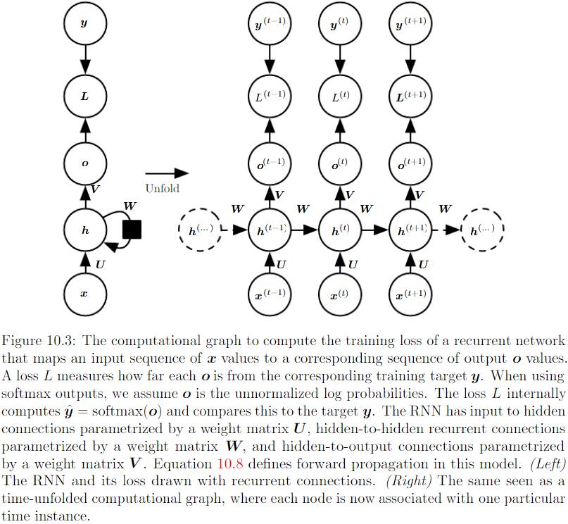
每个时间步都有输出,并且hidden units有循环连接的循环网络:
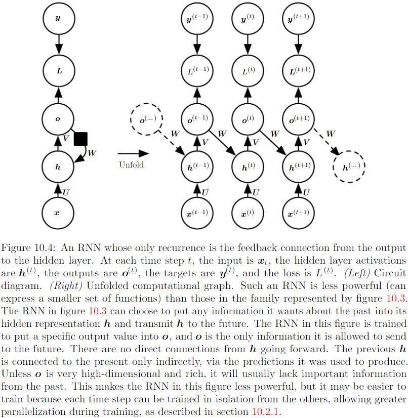
每个时间步都产生一个输出,只有当前时刻的输出到下个时刻的hidden units之间有循环单元:
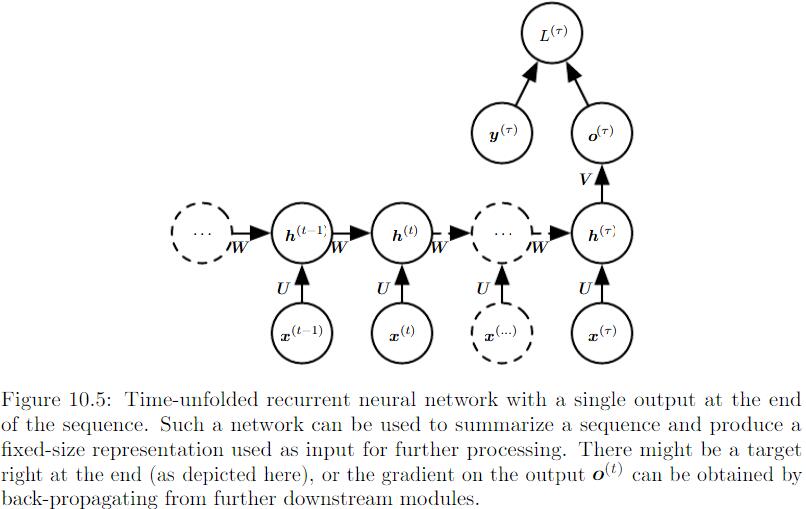
Hidden units之间存在循环连接,但读取整个sequence之后产生单个输出:
表示离散变量的常规方式是把输出 $o$ 作为每个离散变量可能值的非标准化对数概率,然后我们可以应用Softmax处理,得到标准化后的概率输出向量$\hat{y}$。RNN从特定的初始状态$h^{(0)}$开始前向传播。从$t=1$到$t=\tau$的每个时间步,我们应用以下更新方程:
$$
a^{(t)} = Wh^{(t-1)}+Ux^{(t)}+b
$$
$$
h^{(t)}=tanh(a^{(t)})
$$
$$
o^{(t)}=Vh^{(t)}+c
$$
$$
\hat{y}^{(t)}=softmax(o^{(t)})
$$
$U, V, W$分别对应 input layers to hidden layers,hidden layers to output layers,hidden to next hidden layers的连接。该RNN将一个input sequence映射到相同长度的output sequence。与 $x$ 序列配对的 $y$ 的总Loss就是所有时间步的Loss之和。
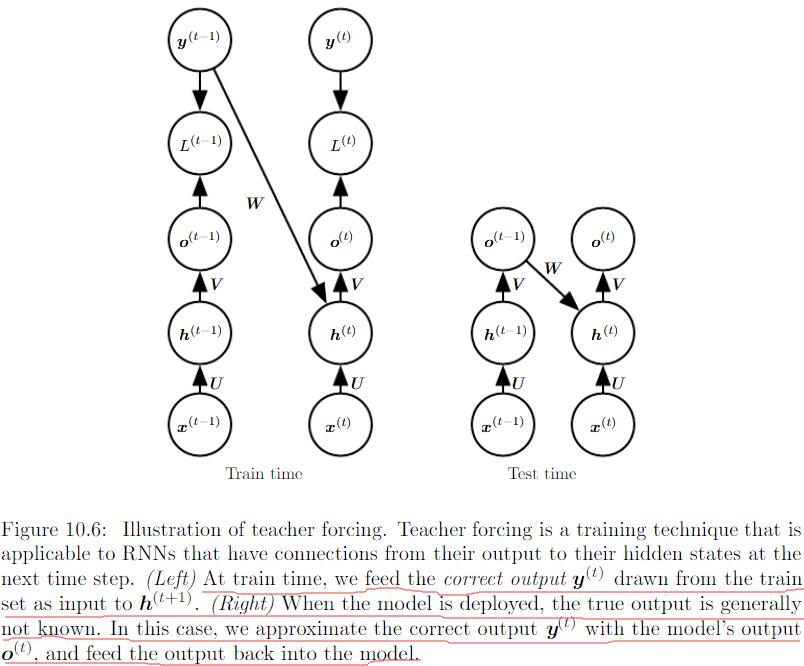
Teacher Forcing and Networks with Output Recurrence
由输出反馈到模型而产生循环连接的model可用teacher forcing进行训练。训练模型时,teacher forcing不再使用最大似然准则,而在时刻 $t+1$ 接收真实值 $y^{(t)}$ 作为输入。条件最大似然准则是:
$$
log p(y^{(1)}, y^{(2)}|x^{(1)},y^{(2)})=log p(y^{(2)}|y^{(1)},x^{(1)},y^{(2)})+log p(y^{(1)}|x^{(1)},y^{(2)})
$$
Computing the Gradient in RNN
以最终的Loss开始,计算:
$\frac{\partial L}{\partial L^{(t)}}=1$
对所有 $i,t$ 关于时间步 $t$ 输出的梯度 $\triangledown_{o^{(t)}}L$ 如下:
$(\triangledown_{o^{(t)}}L)_i=\frac{\partial L}{\partial o_i^{(t)}}=\frac{\partial L}{\partial L^{(t)}} \frac{\partial L^{(t)}}{\partial o_i^{(t)}}=\hat{y}_i^{(t)}-\textbf{1}_{i,y^{(t)}}$
从序列的末尾开始,反向进行计算,在最后的时间步 $\tau, h^{(\tau)}$ 只有 $o^{(\tau)}$ 作为后续结点,因此这个梯度计算很简单:
$\triangledown_{h^{(\tau)}}L=V^T\triangledown_{o^{(\tau)}}L$
然后,我们从时刻$t=\tau -1$到$t=1$反向迭代,通过时间反向传播梯度,注意 $h^{(t)} (t<\tau)$同时具有 $o^{(t)}$ 和 $h^{(t+1)}$两个后续结点。因此,它的梯度如下计算:
$$
\triangledown_{h^{(t)}}L=(\frac{\partial h^{(t+1)}}{\partial h^{(t)}})^T(\triangledown_{h^{(t+1)}}L)+(\frac{\partial o^{(t)}}{\partial h^{(t)}})^T(\triangledown_{o^{(t)}}L)=W^T(\triangledown_{h^{(t+1)}}L)diag(1-(h^{(t+1)})^2)+V^T(\triangledown_{o^{(t)}}L)
$$
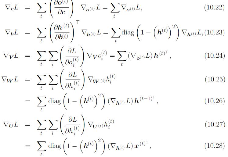
剩下的参数梯度可以由下式给出: