
Introduction
Computer Vision已进入Deep Learning时代,但传统图像特征提取方法依然在很多方向有着不少的应用。毕竟DNN计算复杂度太高,且过于依赖Large Scale Labeled Dataset,所以Deep Learning也并非万能的。本文就传统图像特征提取算子做一下简单的归纳。
本文内容主要来源于TPAMI的一篇文章《TPAMI-A_performance_evaluation_of_local_descriptors》,详情请阅读原文!
Image Descriptors
Image Pixels
简单,但是高维向量带来的复杂计算量。可通过下采样、PCA等方式进行降维。
Distribution-Based Descriptors
A simple descriptor is the distribution of the pixel intensities represented by a histogram.
SIFT
The descriptor is represented by a 3D histogram of gradient locations and orientations; see Fig. 1 for an illustration. The contribution to the locationand orientation bins is weighted by the gradient magnitude. The quantization of gradient locations and orientations makes the descriptor robust to small geometric distortions and small errors in the region detection. Geometric histogram [1] and shape context [3] implement the same idea and are very similar to the SIFT descriptor. Both methods compute a histogram describing the edge distribution in a region. These descriptors were successfully used, for example, for shape recognition of drawings for which edges are reliable features.
EXPERIMENTAL SETUP
Support Regions
Lindeberg [23] has developed a scaleinvariant “blob” detector, where a “blob” is defined by a maximum of the normalized Laplacian in scale-space. Lowe [25] approximates the Laplacian with difference-of-Gaussian (DoG) filters and also detects local extrema in scalespace. Lindeberg and Ga°rding [24] make the blob detector affine-invariant using an affine adaptation process based on the second moment matrix.
Region Detectors
Harris points [15] are invariant to rotation. The support region is a fixed size neighborhood of $41\times 41$ pixels centered at the interest point.
Harris-Laplace regions [29] are invariant to rotation and scale changes. The points are detected by the scale-adapted Harris function and selected in scale-space by the Laplacian- of-Gaussian operator. Harris-Laplace detects cornerlike structures.
Hessian-Laplace regions [25], [32] are invariant to rotation and scale changes. Points are localized in space at the local maxima of the Hessian determinant and in scale at the local maxima of the Laplacian-of-Gaussian. This detector is similar to the DoG approach [26], which localizes points at local scale-space maxima of the difference-of-Gaussian. Both approaches detect similar blob-like structures. However, Hessian-Laplace obtains a higher localization accuracy in scale-space, as DoG also responds to edges and detection is unstable in this case. The scale selection accuracy is also higher than in the case of the Harris-Laplace detector. Laplacian scale selection acts as a matched filter and works better on blob-like structures than on corners since the shape of the Laplacian kernel fits to the blobs. The accuracy of the detectors affects the descriptor performance.
Harris-Affine regions [32] are invariant to affine image transformations. Localization and scale are estimated by the Harris-Laplace detector. The affine neighborhood is determined by the affine adaptation process based on the second moment matrix.
Hessian-Affine regions [33] are invariant to affine image transformations. Localization and scale are estimated by the Hessian-Laplace detector and the affine neighborhood is determined by the affine adaptation process.
Hessian-Affine and Hessian-Laplace detect mainly blob-like structures for which the signal variations lie on the blob boundaries. To include these signal changes into the description, the measurement region is three times larger than the detected region. This factor is used for all scale and affine detectors. All the regions are mapped to a circular region of constant radius to obtain scale and affine invariance. The size of the normalized region should not be too small in order to represent the local structure at a sufficient resolution. In all experiments, this size is arbitrarily set to 41 pixels.
Descriptors
SIFT
SIFT descriptors are computed for normalized image patches with the code provided by Lowe [25]. A descriptor is a 3D histogram of gradient location and orientation, where location is quantized into a $4\times 4$ location grid and the gradient angle is quantized into eight orientations. The resulting descriptor is of dimension 128.
Each orientation plane represents the gradient magnitude corresponding to a given orientation. To obtain illumination invariance, the descriptor is normalized by the square root of the sum of squared components.
Gradient location-orientation histogram (GLOH)
Gradient location-orientation histogram (GLOH) is an extension of the SIFT descriptor designed to increase its robustness and distinctiveness. We compute the SIFT descriptor for a log-polar location grid with three bins in radial direction (the radius set to 6, 11, and 15) and 8 in angular direction, which results in 17 location bins. Note that the central bin is not divided in angular directions. The gradient orientations are quantized in 16 bins. This gives a 272 bin histogram. The size of this descriptor is reduced with PCA. The covariance matrix for PCA is estimated on 47,000 image patches collected from various images (see Section 3.3.1). The 128 largest eigenvectors are used for description.
Shape context
Shape context is similar to the SIFT descriptor, but is based on edges. Shape context is a 3D histogram of edge point locations and orientations. Edges are extracted by the Canny [5] detector. Location is quantized into nine bins of a log-polar coordinate system as displayed in Fig. 1e with the radius set to 6, 11, and 15 and orientation quantized into four bins (horizontal, vertical, and two diagonals). We therefore obtain a 36 dimensional descriptor.
PCA-SIFT
PCA-SIFT descriptor is a vector of image gradients in x and y direction computed within the support region. The gradient region is sampled at $39\times 39$ locations, therefore, the vector is of dimension 3,042. The dimension is reduced to 36 with PCA.
Spin image
Spin image is a histogram of quantized pixel locations and intensity values. The intensity of a normalized patch is quantized into 10 bins. A 10 bin normalized histogram is computed for each of five rings centered on the region. The dimension of the spin descriptor is 50.
Cross correlation
Cross correlation. To obtain this descriptor, the region is smoothed and uniformly sampled. To limit the descriptor dimension, we sample at $9\times 9$ pixel locations. The similarity between two descriptors is measured with cross-correlation.
DISCUSSION AND CONCLUSIONS
In most of the tests, GLOH obtains the best results, closely followed by SIFT. This shows the robustness and the distinctive character of the region-based SIFT descriptor. Shape context also shows a high performance. However, for textured scenes or when edges are not reliable, its score is lower. The best low-dimensional descriptors are gradientmoments and steerable filters. They can be considered as an alternative when the high dimensionality of the histogram-based descriptors is an issue. Differential invariants give significantly worse results than steerable filters, which is surprising as they are based on the same basic components (Gaussian derivatives). The multiplication of derivatives necessary to obtain rotation invariance increases the instability. Cross correlation gives unstable results. The performance depends on the accuracy of interest point and region detection, which decreases for significant geometric transformations. Cross correlation is more sensitive to these errors than other high dimensional descriptors. Regions detected by Hessian-Laplace and Hessian-Affine are mainly blob-like structures. There are no significant signal changes in the center of the blob therefore descriptors perform better on larger neighborhoods. The results are slightly but systematically better on Hessian regions than on Harris regions due to their higher accuracy. The ranking of the descriptors is similar for different matching strategies. We can observe that SIFT gives relatively better results if nearest neighbor distance ratio is used for thresholding. Note that the precision is higher for nearest neighbor based matching than for threshold based matching.
Appendix
颜色直方图
颜色直方图是在许多图像检索系统中被广泛采用的颜色特征。颜色直方图所描述的是不同色彩在整幅图像中所占的比例,而并不关心每种色彩所处的空间位置,即无法描述图像中的对象或物体。颜色直方图特别适于描述那些难以进行自动分割的图像。计算颜色直方图需要将颜色空间划分成若干个小的颜色区间,每个小区间成为直方图的一个 Bin。这个过程称为颜色量化(Color Quantization)。然后,通过计算颜色落在每个小区间内的像素数量可以得到颜色直方图。颜色量化有许多方法,例如向量量化、聚类方法或者神经网络方法。最为常用的做法是将颜色空间的各个分量(维度)均匀地进行划分。选择合适的颜色小区间(即直方图的 Bin)数目和颜色量化方法与具体应用的性能和效率要求有关。一般来说,颜色小区间的数目越多,直方图对颜色的分辨能力就越强。然而,Bin 的数目很大的颜色直方图不但会增加计算负担,也不利于在大型图像库中建立索引。而且对于某些应用来说,使用非常精细的颜色空间划分方法不一定能够提高检索效果,特别是对于不能容忍对相关图像错漏的那些应用。另一种有效减少直方图 Bin 的数目的办法是只选用那些数值最大(即像素数目最多)的 Bin 来构造图像特征,因为这些表示主要颜色的 Bin 能够表达图像中大部分像素的颜色。实验证明这种方法并不会降低颜色直方图的检索效果。事实上,由于忽略了那些数值较小的 Bin,颜色直方图对噪声的敏感程度降低了,检索效果也更好。
灰度直方图
灰度直方图是灰度级的函数,它表示图像中具有每种灰度级的象素的个数,反映图像中每种灰度出现的频率。由于灰度直方图维数最多只能有 256 维,描述能力有限,所以利用灰度直方图表示图像特征的研究比较少。灰度直方图的横坐标是灰度级,纵坐标是该灰度级出现的频率,是图像的最基本的统计特征。
LBP
LBP(Local Binary Pattern,缩写为 LBP)是一种用来描述图像局部纹理特征的算子;显然,它的作用是进行特征提取,而且,提取的特征是图像的纹理特征,并且,是局部的纹理特征。LBP 算子定义为 在 $3\times 3$ 的窗口内,以窗口中心像素为阈值,将相邻的 8 个像素的灰度值与其进行比较,若周围像素值大于中心像素值,则该像素点的位置被标记为 1,否则为 0。这样,3*3 邻域内的 8 个点可产生 8 bit 的无符号数,即得到该窗口的 LBP值,并用这个值来反映该区域的纹理信息。
虽然 LBP 直方图和灰度直方图一样,只有 256 维,但由于灰度直方图是对图像的整体统计,而 LBP 是对图像的局部的特征描述,因此比灰度直方图有更好的特征表达能力。
LBP在纹理分类问题上是一个非常强大的特征;如果局部二值模式特征与方向梯度直方图结合,则可以在一些集合上十分有效的提升检测效果。LBP是一个简单但非常有效的纹理运算符。它将各个像素与其附近的像素进行比较,并把结果保存为二进制数。由于其辨别力强大和计算简单,局部二值模式纹理算子已经在不同的场景下得到应用。LBP最重要的属性是对诸如光照变化等造成的灰度变化的强健性。它的另外一个重要特性是它的计算简单,这使得它可以对图像进行实时分析。
原始的LBP算子定义为在$3\times 3$的窗口内,以窗口中心像素为阈值,将相邻的8个像素的灰度值与其进行比较,若周围像素值大于中心像素值,则该像素点的位置被标记为1,否则为0。这样,$3\times 3$领域内的8个点可产生8bit的无符号数,即得到该窗口的LBP值,并用这个值来反映该区域的纹理信息。如下图所示: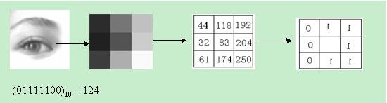
SIFT
SIFT 是一种提取局部特征的算法,在尺度空间寻找极值点,提取位置,尺度,旋转不变量。SIFT 特征是图像的局部特征,其对旋转、尺度缩放、亮度变化保持不变性,对视角变化、仿射变换、噪声也保持一定程度的稳定性。 SIFT 算法步骤:检测尺度空间极值点,精确定位极值点,为每个关键点指定方向参数,关键点描述子的生成。
SIFT检测到的每个关键点有三个信息:位置、所处尺度、方向。
HOG
梯度方向直方图(Histogram of Oriented Gradients,简称 HOG) 描述子是应用在计算机视觉和图像处理领域,用于目标检测的特征描述器。这项技术是用来计算局部图像梯度的方向信息的统计值。
HOG 描述器最重要的思想是:在一副图像中,局部目标的表象和形状(Appearance and Shape)能够被梯度或边缘的方向密度分布很好地描述。具体的实现方法是:首先将图像分成小的连通区域,我们把它叫细胞单元。然后采集细胞单元中各像素点的梯度的或边缘的方向直方图。最后把这些直方图组合起来就可以构成特征描述器。为了提高性能,我们还可以把这些局部直方图在图像的更大的范围内(我们把它叫区间或 Block)进行对比度归一化(Contrast-Normalized),所采用的方法是:先计算各直方图在这个区间(Block)中的密度,然后根据这个密度对区间中的各个细胞单元做归一化。通过这个归一化后,能对光照变化和阴影获得更好的效果。与其他的特征描述方法相比,HOG 描述器后很多优点: 由于 HOG 方法是在图像的局部细胞单元上操作,所以它对图像几何的(Geometric)和光学的(Photometric)形变都能保持很好的不变性。
Reference
- Joost van de Weijer, Cordelia Schmid, Jakob Verbeek, Diane Larlus. Learning Color Names for Real-World Applications. IEEE Transactions on Image Processing, Institute of Electrical and Electronics Engineers, 2009, 18 (7), pp.1512-1523. 10.1109/TIP.2009.2019809. inria-00439284v2
- Navneet Dalal, Bill Triggs. Histograms of Oriented Gradients for Human Detection. International Conference on Computer Vision & Pattern Recognition (CVPR ’05), Jun 2005, San Diego, United States. pp.886–893, 10.1109/CVPR.2005.177. inria-00548512