
Introduction
Feature Engineering 是 Machine Learning 中一个非常非常重要的部分,尤其是工业界。很多时候,为了追求模型的可解释性,效率,我们会更加的倾向于选择合适的特征 + 较为简单的模型,而不会像research那样使用非常复杂的模型来刷分。因此本文主要对ML中常用的特征工程方法做一个简单的介绍。
Numerical Features
Scale
Examples include k-means clustering, nearest neighbors methods, radial basis function (RBF) kernels, and anything that uses the Euclidean distance. For these models and modeling components, it is often a good idea to normalize the features so that the output stays on an expected scale.
Logical functions, on the other hand, are not sensitive to input feature scale. Their output is binary no matter what the inputs are. For instance, the logical AND takes any two variables and outputs 1 if and only if both of the inputs are true. Another example of a logical function is the step function (e.g., is input $x$ greater than 5?). Decision tree models consist of step functions of input features. Hence, models based on space-partitioning trees (decision trees, gradient boosted machines, random forests) are not sensitive to scale**. The only exception is if the scale of the input grows over time, which is the case if the feature is an accumulated count of some sort—eventually it will grow outside of the range that the tree was trained on. If this might be the case, then it might be necessary to rescale the inputs periodically.
Distribution
It’s also important to consider the distribution of numeric features. Distribution summarizes the probability of taking on a particular value. The distribution of input features matters to some models more than others. For instance, the training process of a linear regression model assumes that prediction errors are distributed like a Gaussian. This is usually fine, except when the prediction target spreads out over several orders of magnitude. In this case, the Gaussian error assumption likely no longer holds. One way to deal with this is to transform the output target in order to tame the magnitude of the growth. (Strictly speaking this would be target engineering, not feature engineering.) Log transforms, which are a type of power transform, take the distribution of the variable closer to Gaussian.
Quantization
Raw counts that span several orders of magnitude are problematic for many models. In a linear model, the same linear coefficient would have to work for all possible values of the count. Large counts could also wreak havoc in unsupervised learning methods such as k-means clustering, which uses Euclidean distance as a similarity function to measure the similarity between data points. A large count in one element of the data vector would outweigh the similarity in all other elements, which could throw off the entire similarity measurement. One solution is to contain the scale by quantizing the count. In other words, we group the counts into bins, and get rid of the actual count values. Quantization maps a continuous number to a discrete one. We can think of the discretized numbers as an ordered sequence of bins that represent a measure of intensity.
In order to quantize data, we have to decide how wide each bin should be. The solutions fall into two categories: fixed-width or adaptive. We will give an example of each type.
Fixed-width binning
With fixed-width binning, each bin contains a specific numeric range. The ranges can be custom designed or automatically segmented, and they can be linearly scaled or exponentially scaled. For example, we can group people into age ranges by decade: 0–9 years old in bin 1, 10–19 years in bin 2, etc. To map from the count to the bin, we simply divide by the width of the bin and take the integer part.
It’s also common to see custom-designed age ranges that better correspond to stages of life. When the numbers span multiple magnitudes, it may be better to group by powers of 10 (or powers of any constant): 0–9, 10–99, 100–999, 1000–9999, etc. The bin widths grow exponentially, going from O(10), to O(100), O(1000), and beyond. To map from the count to the bin, we take the log of the count.
Quantile binning
Fixed-width binning is easy to compute. But if there are large gaps in the counts, then there will be many empty bins with no data. This problem can be solved byadaptively positioning the bins based on the distribution of the data. This can be done using the quantiles of the distribution. Quantiles are values that divide the data into equal portions. For example, the median divides the data in halves; half the data points are smaller and half larger than the median. The quartiles divide the data into quarters, the deciles into tenths, etc.
Log Transformation
The log transform is a powerful tool for dealing with positive numbers with a heavy-tailed distribution. (A heavy-tailed distribution places more probability mass in the tail range than a Gaussian distribution.) It compresses the long tail in the high end of the distribution into a shorter tail, and expands the low end into a longer head.
Power Transforms: Generalization of the Log
Transform The log transform is a specific example of a family of transformations known as power transforms. In statistical terms, these are variance-stabilizing transformations. To understand why variance stabilization is good, consider the Poisson distribution. This is a heavy-tailed distribution with a variance that is equal to its mean: hence, the larger its center of mass, the larger its variance, and the heavier the tail. Power transforms change the distribution of the variable so that the variance is no longer dependent on the mean.
A simple generalization of both the square root transform and the log transform is known as the Box-Cox transform:
$$
\tilde{x}=
\begin{cases}
\frac{x^{\lambda}-1}{\lambda} & if \lambda \neq 0,\\
ln(x) & if \lambda = 0
\end{cases}
$$
The Box-Cox formulation only works when the data is positive. For nonpositive data, one could shift the values by adding a fixed constant. When applying the Box-Cox transformation or a more general power transform, we have to determine a value for the parameter $\lambda$. This may be done via maximum likelihood (finding the $\lambda$ that maximizes the Gaussian likelihood of the resulting transformed signal) or Bayesian methods.
Feature Scaling or Normalization
Smooth functions of the input, such as linear regression, logistic regression, or anything that involves a matrix, are affected by the scale of the input. Tree-based models, on the other hand, couldn’t care less. If your model is sensitive to the scale of input features, feature scaling could help. As the name suggests, feature scaling changes the scale of the feature. Sometimes people also call it feature normalization. Feature scaling is usually done individually to each feature.
Min-Max Scaling
$\tilde{x}\frac{x-min(x)}{max(x)-min(x)}$
Standardization (Variance Scaling)
$\tilde{x}=\frac{x-mean(x)}{sqrt{(var(x))}}$
It subtracts off the mean of the feature (over all data points)and divides by the variance. Hence, it can also be called variance scaling. The resulting scaled feature has a mean of 0 and a variance of 1. If the original feature has a Gaussian distribution, then the scaled feature does too.
Use caution when performing min-max scaling and standardization on sparse features. Both subtract a quantity from the original feature value. For min-max scaling, the shift is the minimum over all values of the current feature; for standardization, it is the mean. If the shift is not zero, then these two transforms can turn a sparse feature vector where most values are zero into a dense one. This in turn could create a huge computational burden for the classifier, depending on how it is implemented (not to mention that it would be horrendous if the representation now included every word that didn’t appear in a document!). Bag-of-words is a sparse representation, and most classification libraries optimize for sparse inputs.
$L^2$ Normalization
$\tilde{x}=\frac{x}{||x||_2}$
Feature Selection
Feature selection techniques prune away nonuseful features in order to reduce the complexity of the resulting model. The end goal is a parsimonious model that is quicker to compute, with little or no degradation in predictive accuracy. In order to arrive at such a model, some feature selection techniques require training more than one candidate model. In other words, feature selection is not about reducing training time—in fact, some techniques increase overall training time—but about reducing model scoring time.
Roughly speaking, feature selection techniques fall into three classes:
Filtering
Filtering techniques preprocess features to remove ones that are unlikely to be useful for the model. For example, one could compute the correlation or mutual information between each feature and the response variable, and filter out the features that fall below a threshold. Chapter 3 discusses examples of these techniques for text features. Filtering techniques are much cheaper than the wrapper techniques described next, but they do not take into account the model being employed. Hence, they may not be able to select the right features for the model. It is best to do prefiltering conservatively, so as not to inadvertently eliminate useful features before they even make it to the model training step.
Wrapper methods
These techniques are expensive, but they allow you to try out subsets of features, which means you won’t accidentally prune away features that are uninformative by themselves but useful when taken in combination. The wrapper method treats the model as a black box that provides a quality score of a proposed subset for features. There is a separate method that iteratively refines the subset.
Embedded methods
These methods perform feature selection as part of the model training process. For example, a decision tree inherently performs feature selection because it selects one feature on which to split the tree at each training step. Another example is the regularizer, which can be added to the training objective of any linear model. The regularizer encourages models that use a few features as opposed to a lot of features, so it’s also known as a sparsity constraint on the model. Embedded methods incorporate feature selection as part of the model training process. They are not as powerful as wrapper methods, but they are nowhere near as expensive. Compared to filtering, embedded methods select features that are specific to the model. In this sense, embedded methods strike a balance between computational expense and quality of results.
Categorical Variables: Counting Eggs in the Age of Robotic Chickens
Encoding Categorical Variables
One-Hot Encoding
A better method is to use a group of bits. Each bit represents a possible category. If the variable cannot belong to multiple categories at once, then only one bit in the group can be “on.” This is called one-hot encoding, and it is implemented in scikit-learn as sklearn.preprocessing.OneHotEncoder. Each of the bits is a feature. Thus, a categorical variable with k possible categories is encoded as a feature vector of length k.
Dummy Coding
The problem with one-hot encoding is that it allows for k degrees of freedom, while the variable itself needs only k–1. Dummy coding removes the extra degree of freedom by using only k–1 features in the representation (see Table 5-2). One feature is thrown under the bus and represented by the vector of all zeros. This is known as the reference category. Dummy coding and one-hot encoding are both implemented in Pandas as pandas.get_dummies.
Effect Coding
Yet another variant of categorical variable encoding is effect coding. Effect coding is very similar to dummy coding, with the difference that the reference category is now represented by the vector of all –1’s.
Pros and Cons of Categorical Variable Encodings
One-hot, dummy, and effect coding are very similar to one another. They each have pros and cons. One-hot encoding is redundant, which allows for multiplevalid models for the same problem. The nonuniqueness is sometimes problematic for interpretation, but the advantage is that each feature clearly corresponds to a category. Moreover, missing data can be encoded as the allzeros vector, and the output should be the overall mean of the target variable. Dummy coding and effect coding are not redundant. They give rise to unique and interpretable models. The downside of dummy coding is that it cannot easily handle missing data, since the all-zeros vector is already mapped to the reference category. It also encodes the effect of each category relative to the reference category, which may look strange. Effect coding avoids this problem by using a different code for the reference category, but the vector of all –1’s is a dense vector, which is expensive for both storage and computation. For this reason, popular ML software packages such as Pandas and scikit-learn have opted for dummy coding or one-hot encoding instead of effect coding. All three encoding techniques break down when the number of categories becomes very large. Different strategies are needed to handle extremely large categorical variables.
Dealing with Large Categorical Variables
Existing solutions can be categorized as follows:
- Do nothing fancy with the encoding. Use a simple model that is cheap to train. Feed one-hot encoding into a linear model (logistic regression or linear support vector machine) on lots of machines.
- Compress the features. There are two choices:
- Feature hashing, popular with linear models
- Bin counting, popular with linear models as well as trees
Feature Hashing
The idea of bin counting is deviously simple: rather than using the value of the categorical variable as the feature, instead use the conditional probability of the target under that value. In other words, instead of encoding the identity of the categorical value, we compute the association statistics between that value and the target that we wish to predict. For those familiar with naive Bayes classifiers, this statistic should ring a bell, because it is the conditional probability of the class under the assumption that all features are independent.
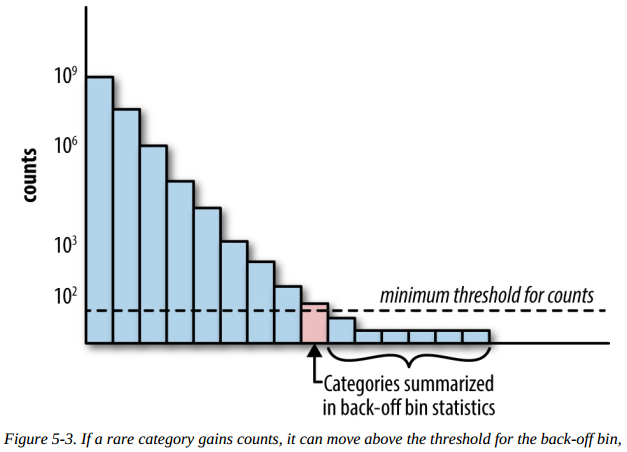
What about rare categories?
One way to deal with this is through back-off, a simple technique that accumulates the counts of all rare categories in a special bin (see Figure 5-3). If the count is greater than a certain threshold, then the category gets its own count statistics. Otherwise, we use the statistics from the back-off bin. This essentially reverts the statistics for a single rare category to the statistics computed on all rare categories. When using the back-off method, it helps to also add a binary indicator for whether or not the statistics come from the back-off bin.
There is another way to deal with this problem, called the count-min sketch (Cormode and Muthukrishnan, 2005). In this method, all the categories, rare or frequent alike, are mapped through multiple hash functions with an output range, m, much smaller than the number of categories, k. When retrieving a statistic, recompute all the hashes of the category and return the smallest statistic. Having multiple hash functions mitigates the probability of collision within a single hash function. The scheme works because the number of hash functions times m, the size of the hash table, can be made smaller than k, the number of categories, and still retain low overall collision probability.
Counts without bounds
If the statistics are updated continuously given more and more historical data, the raw counts will grow without bounds. This could be a problem for the model. A trained model “knows” the input data up to the observed scale.
For this reason, it is often better to use normalized counts that are guaranteed to be bounded in a known interval. For instance, the estimated click-through probability is bounded between [0, 1]. Another method is to take the log transform, which imposes a strict bound, but the rate of increase will be very slow when the count is very large.
Summary
Plain one-hot encoding
Space requirement $O(n)$ using the sparse vector format, where n is the number of data points.
Computation requirement $O(nk)$ under a linear model, where k is the number of categories.
Pros
- Easiest to implement
- Potentially most accurate
- Feasible for online learning
Cons
- Computationally inefficient
- Does not adapt to growing categories
- Not feasible for anything other than linear models
- Requires large-scale distributed optimization with truly
large datasets
Feature hashing
Space requirement $O(n)$ using the sparse matrix format, where n is the number of data points.
Computation requirement $O(nm)$ under a linear or kernel model, where m is the number of hash bins.
Pros
- Easy to implement
- Makes model training cheaper
- Easily adaptable to new categories
- Easily handles rare categories
- Feasible for online learning
Cons
- Only suitable for linear or kernelized models
- Hashed features not interpretable
- Mixed reports of accuracy
Bin-counting
Space requirement $O(n+k)$ for small, dense representation of each data point, plus the count statistics that must be kept for each category.
Computation requirement $O(n)$ for linear models; also usable for nonlinear models such as trees.
Pros
- Smallest computational burden at training time
- Enables tree-based models
- Relatively easy to adapt to new categories
- Handles rare categories with back-off or count-min sketch
- Interpretable
Cons
- Requires historical data
- Delayed updates required, not completely suitable for online
learning - Higher potential for leakage